S35 Accelerator & Detector Physics

Accelerator Physics by Professor Adrian Oeftiger

Lecture 4: Magnets and Focusing

Run this notebook online!

Interact and run this jupyter notebook online:

via the local Physics Jupyterlab service:

via the public mybinder.org service:

Also find this lecture rendered as HTML slides on github $\nearrow$ along with the source repository $\nearrow$.

Run this first!

Imports and modules:

from config import (np, plt, plot_Efield_vs_Ekin, 
                    plot_quadfield, plot_sextfield)
from scipy.constants import m_p, e, c
%matplotlib inline

Refresher!

• beam rigidity equation: $B\rho=p/|q|$
• synchrotron principle, $f_\text{rf}=h\cdot f_\text{rev}$ with harmonic $h\in\mathbb{N}$
• momentum compaction $\alpha_c$ due to path length change with momentum
• phase-slip factor $\eta=\gamma_t^{-2}-\gamma^{-2}$
• transition energy $\gamma_t$
• longitudinal particle tracking equations for synchrotrons
• Hamiltonian landscape for synchrotron motion
• simulation of acceleration ramp, incl. transition crossing:
  "classical" vs. "relativistic" regime and $\varphi_s\mapsto\pi-\varphi_s$ synchronous phase adjustment

Today!

1. Magnetic Fields: Dipoles, Quadrupoles, Sextupoles
2. Linear Transverse Beam Dynamics & Betatron Transfer Matrices
3. Simulations of Betatron Motion

Part I: Magnetic Fields: Dipoles, Quadrupoles, Sextupoles

Magnetic or Electric Fields

The motion of a charged particle in an electric or magnetic field is described by the Lorentz force:

$$\mathbf{F}_L=q(\mathbf{E} + \mathbf{v}\times \mathbf{B})$$

To achieve the same deflection, a 1 T magnetic field corresponds to an equivalent electric field of...

plot_Efield_vs_Ekin();

Electrons have a rest mass of $m_0c^2\approx 511$ keV and protons of $m_0c^2\approx 938$ MeV.

$\leadsto$ Consider an $E$-field of 100 MV/m. At what (low) kinetic energy is a 1 T $B$-field equivalent to this (very high) $E$-field in terms of the Lorentz force? Compare this energy to the energies reached in the accelerator facilities discussed in Lecture 1!

Maxwell Equations: Magnetostatics

$$\left\{\begin{array}\, \nabla \cdot \mathbf{E} &=& \frac{\rho}{\epsilon_0} \\ \nabla \times \mathbf{E} + \frac{\partial\mathbf{B}}{\partial t} &=& \mathbf{0} \\ \nabla \cdot \mathbf{B} &=& 0 \\ \nabla \times \mathbf{B} - \frac{1}{c^2} \frac{\partial\mathbf{E}}{\partial t} &=& \mu_0 \mathbf{j} \end{array}\right.$$

Constant (or adiabatically changing) magnetic fields at beam location in vacuum determined by:

$$\mathbf{j}=0\quad\text{and}\quad\frac{\partial\mathbf{E}}{\partial t}=0\implies\text{magnetostatics: }\left\{\begin{array}\,\nabla\cdot \mathbf{B} &= 0 \\ \nabla \times \mathbf{B}&=0\end{array}\right.$$

Revisited: Beam Rigidity and Circular Orbit

From $F_\text{centrip} = F_\text{L}$, obtained beam rigidity expression $B\rho=p/|q|$ in Lecture 3.

In practical units:

$$p~[\mathrm{GeV}/c]=0.3\,B~[\mathrm{T}]\cdot\rho~[\mathrm{m}]$$

$\implies$ For a circular accelerator or storage ring, use dipole fields $B_y$ to create horizontal closed circular orbit. Typically achieve a dipole filling factor of up to 2/3 of the ring circumference.

$\leadsto$ The 27 km long LHC ring consists of 1232 dipole magnets. What approximate field strength $B_y$ do they provide to maintain this circular orbit at the maximum beam momentum of 7 TeV/$c$?

Multipole Expansion / Beth Representation

Transverse magnetic fields $B_{x,y}$ can be expanded in a multipole series, also known as Beth representation:

$$B_x + iB_y = B_0 \sum\limits_{n=1}^\infty (b_n + ia_n)\cdot (x+iy)^{n-1}$$

The $b_n,a_n$ are the multipole coefficients for normal and skew field components, respectively, and $B_0$ refers to the reference (dipole) field.

$$\begin{align}\, n=1&\text{: dipole} \\ n=2&\text{: quadrupole} \\ n=3&\text{: sextupole} \\ n=4&\text{: octupole} \\ &... \end{align}$$

"Skew" refers to a rotation of the field pattern by half a symmetry period. Consider e.g. a dipole, which has a 180 deg symmetry: a normal dipole with a vertical upright field becomes a skew dipole with a horizontal field (rotated by 180 deg/2 = 90 deg). A skew quadrupole is correspondingly rotated by 45 deg, a skew sextupole by 30 deg, etc.

In the following, consider simplified case in the $y=0$ magnetic "mid-plane": $B_x$ terms disappear and $x\cdot y$ cross-terms vanish.

The $B_y$-field can be Taylor-expanded around reference orbit as

$$\cfrac{B_y}{B\rho} = \underbrace{\phantom{\biggl|}\frac{1}{\rho_0}}\limits_\text{dipole} + \underbrace{\phantom{\biggl|}k\cdot x}\limits_\text{quadrupole} + \underbrace{\phantom{\biggl|}\frac{1}{2!} m x^2}\limits_\text{sextupole} + \underbrace{\phantom{\biggl|}\frac{1}{3!} r x^3}\limits_\text{octupole} + \cdots $$

with the beam rigidity $B\rho=\frac{p}{|q|}$.

Dipole Fields

Const. field in vertical direction $y$ with $b_1=1$ for the main dipoles.

Quadrupole Fields

Quadrupoles provide focusing gradient $G$ for transverse planes.

Main quadrupole magnets are centred on reference orbit such that $B_{y,x}(x=y=0)=0$.

Normal quadrupole field: $\mathbf{B}=\underbrace{B_0\cdot b_2}\limits_{\mathop{\doteq}-G} \cdot \begin{pmatrix} y \\ x \\ 0 \end{pmatrix}$

Skew quadrupole field: $\mathbf{B}=B_0\cdot a_2 \cdot \begin{pmatrix} x \\ -y \\ 0 \end{pmatrix}$

$\leadsto$ Verify that $\nabla\times \mathbf{B}=0$.

plot_quadfield()

Sextupole Fields

Usage: correct chromatic aberration of quadrupoles (dependency on particle's $\delta$, cf. Lecture 6).

Normal sextupole field: $\mathbf{B}=B_0\cdot b_3 \cdot \begin{pmatrix} 2xy \\ x^2-y^2 \\ 0 \end{pmatrix} \quad\implies $ non-linear dynamics!

plot_sextfield()

Part II: Linear Transverse Beam Dynamics
& Betatron Transfer Matrices

Transverse Equations of Motion

Starting from the Lorentz force,

$\cfrac{d\mathbf{p}}{dt}=q\cdot \mathbf{v}\times\mathbf{B}\quad$ with $\quad \mathbf{p}=\gamma m_0\mathbf{v}\quad ,$

and applying the paraxial approximation, $v_z\approx |\mathbf{v}|=\beta c$ as well as $v_x,v_y\ll |\mathbf{v}|$, we find:

$$\implies\left\{\begin{array}\,\gamma m_0\cfrac{d^2x}{dt^2}&=&-q\cdot v_z\cdot B_y\\ \gamma m_0\cfrac{d^2y}{dt^2}&=&+q\cdot v_z\cdot B_x\end{array}\right.$$

Since $\cfrac{d}{dt}=\cfrac{ds}{dt}\,\cfrac{d}{ds}\approx \beta c\cfrac{d}{ds}$, and replacing the beam rigidity expression $p/|q|=B\rho$, the equations of motion for particles in transverse magnetic fields yield

$$\implies \left\{\begin{matrix} \cfrac{d^2x}{ds^2} + \cfrac{B_y}{B\rho} = 0 \\ \cfrac{d^2y}{ds^2} - \cfrac{B_x}{B\rho} = 0 \end{matrix}\right.$$

As long as $B_{y,x}$ depend at max. linearly on $x,y$, these ordinary differential equations are linear.

In a drift space, where $\textbf{B}=0$, particles undergo uniform motion, and the transverse coordinates follow straight lines according to their transverse momenta $x'\doteq dx/ds$ and $y'\doteq dy/ds$:

$$\begin{array}\,x(s)=x_0+x'\cdot s\\ y(s)=y_0+y'\cdot s\end{array}$$

Motion in Quadrupole Magnet

The field in normal quadrupole is given by $B_y=-G\cdot x$ and $B_x=-G\cdot y$. To normalise by momentum, define the quadrupole strength

$$k \doteq - \cfrac{G}{B\rho}$$

where conventionally $k>0$ is referred to as a (horizontally) focusing magnet. The equations of motion read

$$\left\{\begin{matrix}\, x'' + k\cdot x &= 0 \\ y'' - k\cdot y &= 0 \end{matrix}\right.$$

with the usual harmonic oscillator solutions: $\cos,\sin$ for stable $u''=-|k|u$ and hyperbolic $\cosh,\sinh$ for unstable $u''=+|k|u$ (with $u=x,y$).

$\implies$ in a quadrupole, one direction always focuses while the other direction defocuses!

Motion in Dipole Magnet

Consider $\Delta s$ long sector dipole magnet (reference orbit enters perpendicularly) with bending angle $\theta$ and bending radius $\rho_0\approx \Delta s/\theta$.

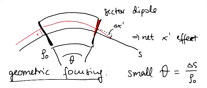
$\implies$ a particle entering with an offset $x$ experiences a net focusing kick, i.e. negative angle $\Delta x'$:

$$\Delta x'= -\cfrac{x}{\rho_0}\cdot \theta = -\cfrac{x}{\rho_0^2}\cdot \Delta s$$

This geometric focusing effect is the result of a longer path length in the dipole field for positive $x$, which yields the following equations of motion in a dipole field:

$$\left\{\begin{matrix}\, x'' + \cfrac{1}{\rho_0{}^2} \cdot x &= 0 \\ y'' &= 0\end{matrix}\right.$$

The horizontal plane corresponds to a harmonic oscillator solution, while the vertical plane corresponds to a drift section.

Hill Differential Equation

Piecing together drifts, normal dipoles and normal quadrupoles to a magnet sequence, the lattice of the accelerator, one obtains the Hill equation

$$\left\{\begin{matrix}\, x'' &\mathop{+}\, \left(\cfrac{1}{\rho_0^2(s)} + k(s)\right)&\mathop{\cdot} x = 0 \\ y'' &\mathop{-} k(s)&\mathop{\cdot} y = 0 \end{matrix}\right.$$

where the dipole curvature radius $\rho_0(s)$ and the quadrupole strength $k(s)$ are typically piecewise constant. Solutions describe the so-called betatron motion in the transverse planes.

$\implies$ Use transverse matrix formalism for each (linear) magnet, the betatron transport matrices $\mathcal{M}$, to advance phase space coordinates through each element from $s_0$ to $s_0+s$:

$$\begin{pmatrix} x \\ x' \end{pmatrix}_{s_0+s} = \mathcal{M}(s_0+s, s_0) \begin{pmatrix} x \\ x' \end{pmatrix}_{s_0}$$

Betatron Transfer Matrices I

A drift section: $$\mathcal{M}_\text{drift} = \begin{pmatrix}\,1 &s \\ 0 & 1\end{pmatrix}$$

A thick dipole magnet: $$\mathcal{M}_\text{dipole}^x = \begin{pmatrix}\,\cos\left(\frac{s}{\rho_0}\right) &\rho_0 \sin\left(\frac{s}{\rho_0}\right) \\ -\frac{1}{\rho_0}\sin\left(\frac{s}{\rho_0}\right) & \cos\left(\frac{s}{\rho_0}\right)\end{pmatrix} \qquad \text{and}\qquad \mathcal{M}_\text{dipole}^{y} = \mathcal{M}_\text{drift} $$

Betatron Transfer Matrices II

A thick quadrupole magnet:

$$\mathcal{M}^\text{foc}_\text{quadrupole} = \begin{pmatrix}\,\cos(\sqrt{|k|}\cdot s) & \frac{1}{\sqrt{|k|}}\sin(\sqrt{|k|}\cdot s) \\ -\sqrt{|k|} \sin(\sqrt{|k|}\cdot s) & \cos(\sqrt{|k|}\cdot s) \end{pmatrix} $$

$$\mathcal{M}^\text{defoc}_\text{quadrupole} = \begin{pmatrix}\,\cosh(\sqrt{|k|}\cdot s) & \frac{1}{\sqrt{|k|}}\sinh(\sqrt{|k|}\cdot s) \\ \sqrt{|k|} \sinh(\sqrt{|k|}\cdot s) & \cosh(\sqrt{|k|}\cdot s) \end{pmatrix}$$

where a focusing quadrupole $k>0$ uses $\mathcal{M}^\text{foc}_\text{quadrupole}$ for the $x$-plane and $\mathcal{M}^\text{defoc}_\text{quadrupole}$ for the $y$-plane. Vice versa for a defocusing quadrupole.

def M_drift(L):
    return np.array([
        [1, L],
        [0, 1]
    ])

def M_dip_x(L, rho0):
    return np.array([
        [np.cos(L / rho0), rho0 * np.sin(L / rho0)],
        [-1 / rho0 * np.sin(L / rho0), np.cos(L / rho0)]
    ])

def M_dip_y(L, rho0):
    return M_drift(L)

def M_quad_x(L, k):
    ksq = np.sqrt(k + 0j)
    return np.array([
        [np.cos(ksq * L), 1 / ksq * np.sin(ksq * L)],
        [-ksq * np.sin(ksq * L), np.cos(ksq * L)]
    ]).real

def M_quad_y(L, k):
    ksq = np.sqrt(k + 0j)
    return np.array([
        [np.cosh(ksq * L), 1 / ksq * np.sinh(ksq * L)],
        [ksq * np.sinh(ksq * L), np.cosh(ksq * L)]
    ]).real

def track(M, u, up):
    '''Apply M to each individual [u;up] vectors value.'''
    return np.einsum('ij,...j->i...', M, np.vstack((u, up)).T)

Thin Approximation

For very short lengths of the magnets $L\rightarrow 0$, one can derive the following triangular matrices under the so-called thin approximation $f=\lim\limits_{L\rightarrow 0} \cfrac{1}{|k|\cdot L}$:

$$\mathcal{M}^\text{foc}_\text{thin-quadrupole} = \begin{pmatrix}\,1 & 0 \\ -\frac{1}{f} & 1 \end{pmatrix}$$

$$\mathcal{M}^\text{defoc}_\text{thin-quadrupole} = \begin{pmatrix}\,1 & 0 \\ \frac{1}{f} & 1 \end{pmatrix}$$

as well as

$$\mathcal{M}^\text{x}_\text{thin-dipole} = M_\text{drift}$$

Thin Sextupole Kick

The motion through a regular sextupole magnet of strength $m$ and length $L$ cannot be represented by a (betatron) matrix since the magnetic field is non-linear.

In thin approximation, an infinitesimally long sextupole magnet of integrated strength $mL$ applies only an update of the momentum (angle):

$$\left\{\begin{matrix}\, x'|_\text{after} &= x'|_\text{before} \,+ &\frac{1}{2} m (y^2 - x^2)\cdot L \\ y'|_\text{after} &= y'|_\text{before} \,+ &m \cdot x \cdot y \cdot L \end{matrix}\right.$$

def track_sext_4D(x, xp, y, yp, mL):
    xp += 0.5 * mL * (y * y - x * x)
    yp += mL * x * y
    return x, xp, y, yp

Part III: Simulations of Betatron Motion

Simulation Exercises

1. Simulating a drift:

np.random.seed(12345)

N = 100
sig_x = 5e-3
sig_xp = 2e-3

x = np.random.normal(0, sig_x, N)
xp = np.random.normal(0, sig_xp, N)

ds = 0.01

D = M_drift(ds)

plt.scatter(x, xp, c='C0', s=10, marker='.')
plt.title('Initial phase space distribution', y=1.04)
plt.xlabel('$x$')
plt.ylabel("$x'$");

for s in np.arange(-1, 1, ds):
    x, xp = track(D, x, xp)
    plt.scatter(np.ones(N) * s, x, c='C0', s=1, marker='.')
plt.title('Particle motion along path length', y=1.04)
plt.xlabel('$s$')
plt.ylabel('$x$');

plt.scatter(x, xp, c='C0', s=10, marker='.')
plt.title('Final phase space distribution', y=1.04)
plt.xlabel('$x$')
plt.ylabel("$x'$");

Same simulation again with correlated $x, x'$:

$\implies$ demonstrates the eventual divergence after long enough drifts

np.random.seed(12345)

N = 100
sig_x = 5e-3
sig_xp = 2e-3

x = np.random.normal(0, sig_x, N)
xp = np.random.normal(0, sig_xp / 2, N) - x * sig_x / sig_xp * 0.4

ds = 0.01

D = M_drift(ds)

plt.scatter(x, xp, c='C0', s=10, marker='.')
plt.title('Initial phase space distribution', y=1.04)
plt.xlabel('$x$')
plt.ylabel("$x'$");

for s in np.arange(-1, 1, ds):
    x, xp = track(D, x, xp)
    plt.scatter(np.ones(N) * s, x, c='C0', s=1, marker='.')
plt.title('Particle motion along path length', y=1.04)
plt.xlabel('$s$')
plt.ylabel('$x$');

$\implies$ Particles drift in straight lines forward and backward along $x$ depending on their momentum (angle) $x'$!

plt.scatter(x, xp, c='C0', s=10, marker='.')
plt.title('Final phase space distribution', y=1.04)
plt.xlabel('$x$')
plt.ylabel("$x'$");

2. Simulating a quadrupole in focusing plane:

np.random.seed(12345)

N = 100
sig_x = 5e-3
sig_xp = 2e-3

x = np.random.normal(0, sig_x, N)
xp = np.random.normal(0, sig_xp, N)

ds = 0.01

Qx = M_quad_x(ds, 10)

plt.scatter(x, xp, c='C0', s=10, marker='.')
plt.title('Initial phase space distribution', y=1.04)
plt.xlabel('$x$')
plt.ylabel("$x'$");

for s in np.arange(-1, 1, ds):
    x, xp = track(Qx, x, xp)
    plt.scatter(np.ones(N) * s, x, c='C0', s=1, marker='.')
plt.title('Particle motion along path length', y=1.04)
plt.xlabel('$s$')
plt.ylabel('$x$');

$\implies$ The distribution of particles is nicely contained within a certain amplitude: focused beam

plt.scatter(x, xp, c='C0', s=10, marker='.')
plt.title('Final phase space distribution', y=1.04)
plt.xlabel('$x$')
plt.ylabel("$x'$");

$\leadsto$ Is it possible to deliver stable beams with a storage ring consisting only of focusing quadrupoles?

3. Simulating a quadrupole in defocusing plane:

np.random.seed(12345)

N = 100
sig_x = 5e-3
sig_xp = 2e-3

x = np.random.normal(0, sig_x, N)
xp = np.random.normal(0, sig_xp, N)

Note the negative sign for $k$ to obtain defocusing in the horizontal plane:

ds = 0.01

Qx = M_quad_x(ds, -10)

plt.scatter(x, xp, c='C0', s=10, marker='.')
plt.title('Initial phase space distribution', y=1.04)
plt.xlabel('$x$')
plt.ylabel("$x'$");

for s in np.arange(-1, 1, ds):
    x, xp = track(Qx, x, xp)
    plt.scatter(np.ones(N) * s, x, c='C0', s=1, marker='.')
plt.title('Particle motion along path length', y=1.04)
plt.xlabel('$s$')
plt.ylabel('$x$');

plt.scatter(x, xp, c='C0', s=10, marker='.')
plt.title('Final phase space distribution', y=1.04)
plt.xlabel('$x$')
plt.ylabel("$x'$");

$\implies$ The issue with a constant, continuous quadrupole field is that it focuses in one plane while defocusing in the other!

4. Stabilising the Transverse Motion:

$\leadsto$ Can you think of a way how to combine quadrupole magnets in a lattice that provides net focusing in both transverse planes?

np.random.seed(12345)

N = 100
sig_x = 5e-3
sig_xp = 3e-4

x = np.random.normal(0, sig_x, N)
xp = np.random.normal(0, sig_xp, N) + 0.15 * x

Choose the focusing strengths $k$ of two consecutive quadrupoles:

ds = 0.1
k1 = 0.2
k2 = -0.2#fill me

D = M_drift(ds)
Q1x = M_quad_x(ds, k=k1)
Q2x = M_quad_x(ds, k=k2)

plt.scatter(x, xp, c='C0', s=10, marker='.')
plt.title('Initial phase space distribution', y=1.04)
plt.xlabel('$x$')
plt.ylabel("$x'$");

We assume a total beam line length of 10m and a length of each quadrupole magnet of 1m.

Suppose you place a first focusing quadrupole after 2m of drift – how would you power a second quadrupole located down the line at 7m? The lattice looks like "0-F-0-?-0" with "F" for focusing and "D" for defocusing quadrupole.

Tracking particles in the horizontal plane first, starting with a drift:

# drift
for s in np.arange(0, 2.0001, ds)[1:]:
    x, xp = track(D, x, xp)
    plt.scatter(np.ones(N) * s, x, c='C0', s=1, marker='.')
# first quad
for s in np.arange(2, 3.0001, ds)[1:]:
    x, xp = track(Q1x, x, xp)
    plt.scatter(np.ones(N) * s, x, c='C0', s=1, marker='.')
# drift
for s in np.arange(3, 7.0001, ds)[1:]:
    x, xp = track(D, x, xp)
    plt.scatter(np.ones(N) * s, x, c='C0', s=1, marker='.')
# second quad
for s in np.arange(7, 8.0001, ds)[1:]:
    x, xp = track(Q2x, x, xp)
    plt.scatter(np.ones(N) * s, x, c='C0', s=1, marker='.')
# drift
for s in np.arange(8, 10.0001, ds)[1:]:
    x, xp = track(D, x, xp)
    plt.scatter(np.ones(N) * s, x, c='C0', s=1, marker='.')
plt.title('Particle motion along path length', y=1.04)
plt.xlabel('$s$')
plt.ylabel('$x$');

plt.scatter(x, xp, c='C0', s=10, marker='.')
plt.title('Final phase space distribution', y=1.04)
plt.xlabel('$x$')
plt.ylabel("$x'$");

What about the vertical plane now? The quadrupoles have their focusing reversed: a quadrupole focusing in the horizontal plane defocuses vertically. A lattice with the sequence "0-F-0-D-0" in the horizontal plane appears as "0-D-0-F-0" in the vertical plane:

sig_y = 5e-3
sig_yp = 3e-4

y = np.random.normal(0, sig_y, N)
yp = np.random.normal(0, sig_yp, N) - 0.15 * y

Q1y = M_quad_y(ds, k1)
Q2y = M_quad_y(ds, k2)

# drift
for s in np.arange(0, 2.0001, ds)[1:]:
    y, yp = track(D, y, yp)
    plt.scatter(np.ones(N) * s, y, c='C0', s=1, marker='.')
# first quad
for s in np.arange(2, 3.0001, ds)[1:]:
    y, yp = track(Q1y, y, yp)
    plt.scatter(np.ones(N) * s, y, c='C0', s=1, marker='.')
# drift
for s in np.arange(3, 7.0001, ds)[1:]:
    y, yp = track(D, y, yp)
    plt.scatter(np.ones(N) * s, y, c='C0', s=1, marker='.')
# second quad
for s in np.arange(7, 8.0001, ds)[1:]:
    y, yp = track(Q2y, y, yp)
    plt.scatter(np.ones(N) * s, y, c='C0', s=1, marker='.')
# drift
for s in np.arange(8, 10.0001, ds)[1:]:
    y, yp = track(D, y, yp)
    plt.scatter(np.ones(N) * s, y, c='C0', s=1, marker='.')
plt.title('Particle motion along path length', y=1.04)
plt.xlabel('$s$')
plt.ylabel('$y$');

$\implies$ One can ensure quasi-harmonic motion in both (!) transverse planes! Transverse confinement of beam by alternating-gradient (AG) focusing over such a "FODO cell"! This is the principle behind synchrotrons! (We will investigate this in more detail in lecture 5.)

How does this look like over longer time scales? Let us build the one-cell matrix and track over many lattice periods:

M_cell = M_drift(2) # drift
M_cell = M_cell.dot(M_quad_x(1, k1)) # focusing quad
M_cell = M_cell.dot(M_drift(4)) # drift
M_cell = M_cell.dot(M_quad_x(1, k2)) # defocusing quad
M_cell = M_cell.dot(M_drift(2)) # drift

n_cells = 100

np.random.seed(12345)

N = 100
sig_x = 5e-3
sig_xp = 3e-4

x = np.random.normal(0, sig_x, N)
xp = np.random.normal(0, sig_xp, N)

for i in range(n_cells):
    x, xp = track(M_cell, x, xp)
    
    plt.scatter(np.ones(N) * i, x, c='C0', s=1, marker='.')
    plt.scatter([i], [x[-1]], c='r', s=10, marker='.')
plt.title('Particle motion over many periods', y=1.04)
plt.xlabel('Cells')
plt.ylabel('$x$');

$\implies$ We observe regular motion, and amplitudes remain bound! This indicates that the magnet configuration is stable and the beam is well confined over long time scales!

What about the phase-space trajectories at this position in the lattice (a Poincaré section)?

for i in range(n_cells):
    x, xp = track(M_cell, x, xp)
    plt.scatter(x[::10], xp[::10], c='C0', s=10, marker='.')
plt.title('Poincaré map', y=1.04)
plt.xlabel('$x$')
plt.ylabel("$x'$");

$\implies$ The closed ellipses indicate linear bound (i.e. stable) motion!

5. What happens for increasingly strong $k$ in FODO cells?

$\leadsto$ Vary the quadrupole strength $k$ and observe the effect of increasing its value!

k = 0.431#fill me 
#0.431
k1 = k
k2 = -k

M_cell = M_drift(2) # drift
M_cell = M_cell.dot(M_quad_x(1, k1)) # focusing quad
M_cell = M_cell.dot(M_drift(4)) # drift
M_cell = M_cell.dot(M_quad_x(1, k2)) # defocusing quad
M_cell = M_cell.dot(M_drift(2)) # drift

n_cells = 100

N = 100
sig_x = 5e-3
sig_xp = 3e-4

x = np.random.normal(0, sig_x, N)
xp = np.random.normal(0, sig_xp, N)

for i in range(n_cells):
    x, xp = track(M_cell, x, xp)
    plt.scatter(np.ones(N) * i, x, c='C0', s=1, marker='.')
    plt.scatter([i], [x[-1]], c='r', s=10, marker='.')
plt.title('Poincaré map', y=1.04)
plt.xlabel('Cells')
plt.ylabel('$x$');

$\implies$ The motion can become unstable for too strong focusing strengths $k$!

"Haste Makes Waste"

image by G. Xia

$\implies$ What about the eigenvalues of the one-cell matrix?

Solve the characteristic polynomial of the matrix, $\det(\mathcal{M}-\lambda\mathbb{1}) = 0$ for $\lambda$:

np.linalg.eigvals(M_cell)

array([-0.87523826, -1.14254604])

$\implies$ We find one $|\lambda| > 1$! If one absolute eigenvalue becomes larger than unity, the magnet configuration becomes unstable! That explains the observed beam instability and exponential divergence here!

What happens to a single particle in phase space on the Poincaré section?

for i in range(10):
    x, xp = track(M_cell, x, xp)
    plt.scatter(x[0], xp[0], c='C0', s=10, marker='.')
plt.title('Poincaré map', y=1.04)
plt.xlabel('$x$')
plt.ylabel("$x'$");

$\leadsto$ Compare this to the stable phase-space portrait before! Can you explain what happens?

Summary

• magnetic fields to deflect particles in the transverse plane (vs. electric fields)
• multipole representation (normal and skew coefficients $b_n,a_n$)
• dipole, quadrupole, sextupole magnetic fields
• equation of motion in magnetic fields (after paraxial approximation)
• Hill differential equation
• betatron matrices for transport (solution to e.o.m.)

---

• drifts: divergence
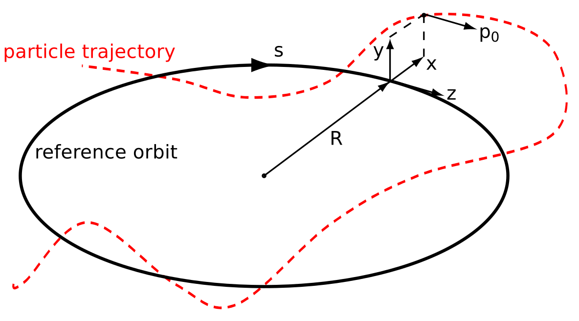
• dipoles: bending included in Frenet-Serret coordinate system, geometric focusing
• quadrupoles: focus in one plane while defocusing in the other

6. Bonus: Simulating a FODO cell with a sextupole:

We go back to the stable FODO cell configuration and add a thin sextupole magnet after 1/4 of the lattice, between the first focusing and the second defocusing quadrupole!

The sextupole kick provides a non-linearity in the potential that confines the particles. At large enough amplitude, the non-linear term dominates and the particles are no longer bound / confined!

We need to track in 4D phase space (full transverse plane with both $x$ and $y$) as the sextupole provides coupling terms:

np.random.seed(12345)

We need a first matrix 1/4 of the cell until the sextupole, once for the $x$ (M_cell_x_1) and another one for the $y$ plane (M_cell_y_1). Then a second matrix each to track $x$ and $y$ for the remaining 3/4 of the cell (M_cell_x_2, M_cell_y_2):

k = 0.2
mL = 1.8

# horizontal plane:
M_cell_x_1 = M_quad_x(0.5, k) # 1/2 focusing quad
M_cell_x_1 = M_cell_x_1.dot(M_drift(2)) # drift
## here is where the sextupole sits
M_cell_x_2 = M_drift(2) # drift
M_cell_x_2 = M_cell_x_2.dot(M_quad_x(1, -k)) # defocusing quad
M_cell_x_2 = M_cell_x_2.dot(M_drift(4)) # drift
M_cell_x_2 = M_cell_x_2.dot(M_quad_x(0.5, k)) # 1/2 focusing quad

# vertical plane:
M_cell_y_1 = M_quad_y(0.5, k) # 1/2 focusing quad
M_cell_y_1 = M_cell_y_1.dot(M_drift(2)) # drift
## here is where the sextupole sits
M_cell_y_2 = M_drift(2) # drift
M_cell_y_2 = M_cell_y_2.dot(M_quad_y(1, -k)) # defocusing quad
M_cell_y_2 = M_cell_y_2.dot(M_drift(4)) # drift
M_cell_y_2 = M_cell_y_2.dot(M_quad_y(0.5, k)) # 1/2 focusing quad

n_cells = 1000

Initialise the transverse particle distribution:

N = 100
sig_x = 5e-3
sig_xp = 3e-4
sig_y = 5e-3
sig_yp = 3e-4

x = np.random.normal(0, sig_x, N)
xp = np.random.normal(0, sig_xp, N)
y = np.random.normal(0, sig_x, N)
yp = np.random.normal(0, sig_xp, N)

Let us record the horizontal phase-space coordinates during the tracking:

rec_x = np.zeros((n_cells, N), dtype=x.dtype)
rec_xp = np.zeros_like(rec_x)

Let us set the last particle to the same phase-space coordinates as the first particle up to a very small epsilon, for later:

x[-1] = x[0]
xp[-1] = xp[0]
y[-1] = y[0]
yp[-1] = yp[0] * 1.001

Let's go, the full 4D tracking loop comes here:

for i in range(n_cells):
    # initial 1/4 of the cell
    x, xp = track(M_cell_x_1, x, xp)
    y, yp = track(M_cell_y_1, y, yp)
    # sextupole
    x, xp, y, yp = track_sext_4D(x, xp, y, yp, mL)
    # remaining 3/4 of the cell
    x, xp = track(M_cell_x_2, x, xp)
    y, yp = track(M_cell_y_2, y, yp)
    
    plt.scatter(np.ones(N) * i, x, c='C0', s=1, marker='.')
    plt.scatter([i], [x[-1]], c='r', s=10, marker='.')
    
    rec_x[i] = x
    rec_xp[i] = xp
plt.xlabel('Cells')
plt.ylabel('$x$');

How does the horizontal phase space (Poincaré map) look like?

for i in range(n_cells):
    plt.scatter(rec_x[:100,::10], rec_xp[:100,::10], c='C0', s=1, marker='.')
plt.title('Poincaré map', y=1.04)
plt.xlabel('$x$')
plt.ylabel("$x'$");

$\implies$ Single particles do not maintain the same (linear) amplitude (radius in $x-x'$) during the tracking!

A single particle motion in phase space looks like this:

plt.plot(rec_x[:, 0])
plt.xlabel('Turns')
plt.ylabel('$x$');

$\implies$ Distorted regular motion (see the asymmetry between positive and negative $x$ values in the oscillation), the particle is still bound but the sextupole deforms the phase-space topology from the regular circles we observed for purely linear tracking.

Remember, the last particle was just a copy from the first particle with a slightly increased $y'$ value. Let us investigate the difference in their horizontal position during the tracking:

plt.plot(np.abs(rec_x[:,0] - rec_x[:,-1]))
plt.yscale('log')
plt.xlabel('Turns')
plt.ylabel(r'$|\Delta x|$');

$\implies$ For finite sextupole strength, we observe on average an exponential increase. This is an early indicator of deterministic chaos (a positive maximum "Lyapunov exponent").

All in all, the thin sextupole magnet in the lattice

• provides a non-linearity in the potential which the particles see
• distorts the regular motion in phase-space
• leads to a change of the (linear) amplitude in phase space
• provides deterministic chaos, in particular at larger amplitudes (positive Lyapunov exponent!)

$\leadsto$ Repeat this exercise with zero sextupole strength $m=0$ to confirm these insights for yourself!

Hint: in order to observe a meaningful result in the last plot, add a factor * 1.001 to xp for the last particle to see an effect. Due to the absent coupling between $x$ and $y$, there will be no difference in the $x$ motion of both particles without the sextupole!