S35 Accelerator & Detector Physics
Accelerator Physics by Professor Adrian Oeftiger
Lecture 3: Transition Energy
Run this notebook online!
Interact and run this jupyter notebook online:
Also find this lecture rendered as HTML slides on github $\nearrow$ along with the source repository $\nearrow$.
Run this first!
Imports and modules:
from config import (np, plt, plot_rfwave, tqdm, trange, )
from scipy.constants import m_p, e, c
%matplotlib inline
Refresher!
- Lorentz force, only longitudinal $E_z$ field component can accelerate
- energy gain in rf cavity: synchronous particle and real particles
- linacs
- phase focusing and stability $=$ bunching
- longitudinal particle tracking equations for linacs
Today!
- Synchrotrons
- Momentum compaction and phase slippage
- Transition energy
- Hamiltonian for longitudinal dynamics
- Simulation of CERN Proton Synchrotron
Part I: Circular Accelerator Concepts
... or how Einstein's relativity hits back!Beam rigidity
Constant (dipole) magnetic field $B$ guides reference particle on circular trajectory with bending radius $\rho$:
$$\begin{align} F_\text{centrip} &= F_\text{L} \\ \frac{\gamma m_0 v^2}{\rho} &= |q| v B \end{align}$$
Synchrotron
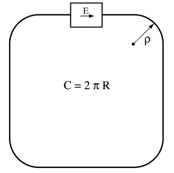
- ring with a constant reference orbit of circumference $C$,
determined by the dipole magnets (defining the beam rigidity) - RF systems powered at revolution frequency $f_{\text{rev}}$
or integer multiple of it ("harmonic" $h$): synchronisation!
$$\begin{align} f_{\text{rev}} &= \frac{\beta c}{C} \\ f_{\text{rf}} &\stackrel{!}{=} h\,f_{\text{rev}} \end{align}$$
$\implies$ $h$ synchronous particles moving along reference orbit! To accelerate them and for longitudinal phase focusing around them, apply $E_z$ in RF cavity!
$\implies$ only works with AC field! Why not DC field across cavity gap?
image by A. Chance and N. Pichoff
Acceleration in Synchrotron
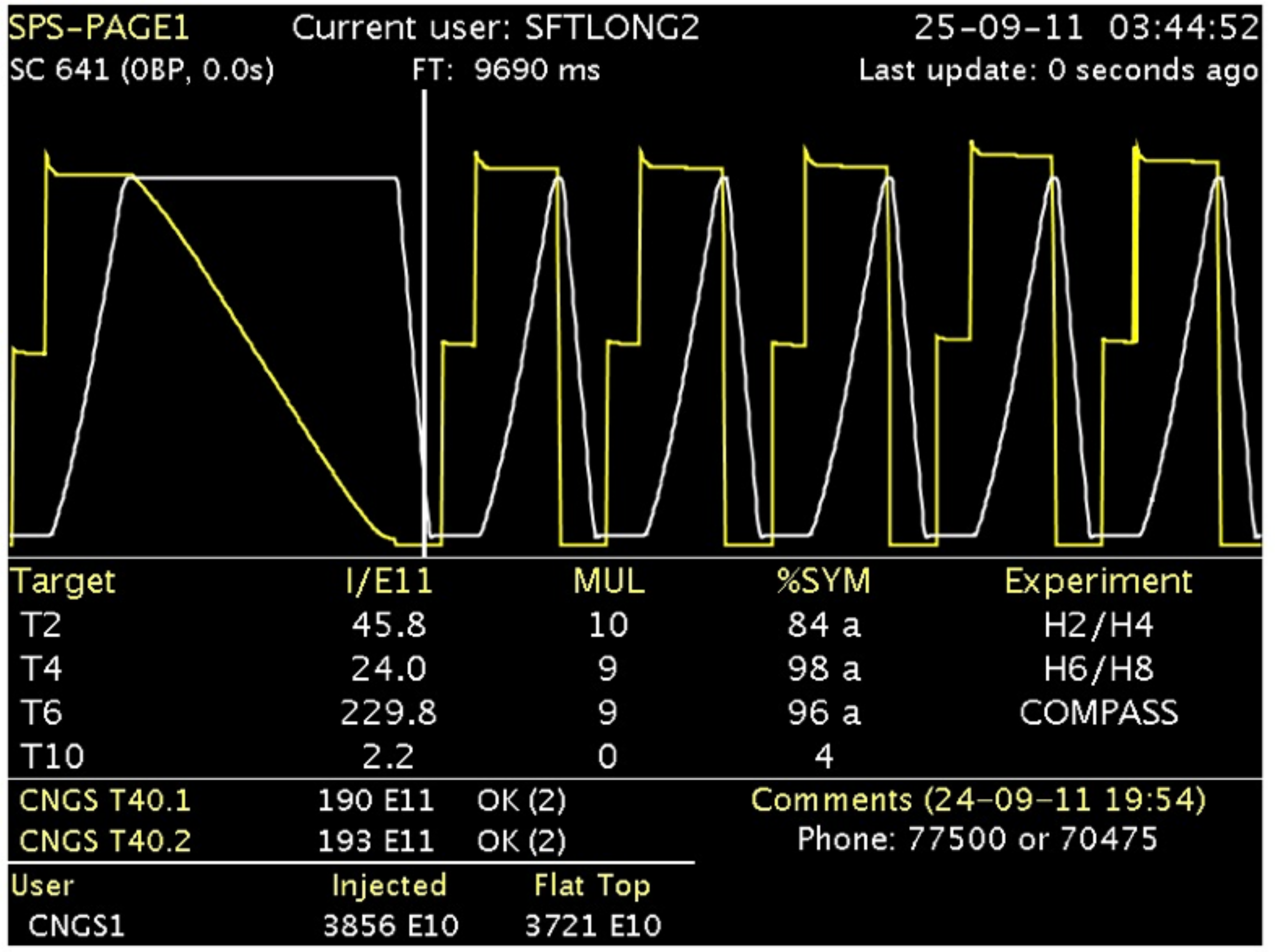
Require (dipole) magnetic fields to synchronise with increasing momentum!
$$\underbrace{\dot{B}}\limits_{=\frac{dB}{dt}}=\frac{\dot{p}}{|q|\rho}$$
$\implies$ synchrotrons "cycle": magnets ramp up fields for acceleration (and back down to inject next beam)
image from CERN Vistars
Mechanism behind Synchrotron
Conceptual "flow chart" of synchrotron operation principle:
- dipole field $B$ increase
- thus, bending radius $\rho$ decrease
- thus, reference orbit length decrease
- thus, synchronous phase $\varphi_s$ decrease (earlier arrival of synchronous particle)
- thus, reference energy/momentum increase (finite RF voltage!)
- thus, back to synchronism (possibly shorter equilibrium reference orbit)
$\implies$ typically magnetic field ramp $\dot{B}$ is slow enough
$\implies$ adiabatic acceleration, particles remain focused around synchronous particle
Off-momentum Trajectory
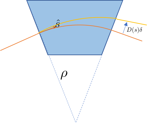
image by Y. Hao

image by BR84, Wikimedia
Particles with higher momentum, $\delta = \Delta p/p_0 > 0$, than the reference particle are bent less (larger $p$ $\implies$ larger $\rho$)!
$$\implies d\ell = \left(1 + \frac{x}{\rho(s)}\right) ds$$
$\implies$ larger equilibrium orbit around the machine for fixed dipole fields $B$!
Can describe this horizontal offset $x$ due to momentum offset $\delta$ by dispersion function $D_x(s)$ (more details later in lecture 6):
$$x(s) = D_x(s) \delta$$
Integrating around machine to get full orbit length:
$$\ell_\text{tot} = \oint d\ell = \underbrace{\oint ds}\limits_{\mathop{\equiv} C} + \delta \oint ds\,\frac{D_x(s)}{\rho(s)}$$
Momentum Compaction Factor I
Relative difference in path length $\Delta C/C = (\ell_\text{tot} - C)/C$ around the ring compared to synchronous particle is therefore:
$$\frac{\Delta C}{C} = \delta~ \underbrace{\frac{1}{C} \oint ds\,\frac{D_x(s)}{\rho(s)}}\limits_{\mathop{\doteq}\alpha_c} = \alpha_c \frac{\Delta p}{p}$$
The momentum compaction factor expresses "how much longer the path length around the ring becomes for higher momenta"!
Momentum Compaction Factor II
$\rho=\infty$ in straight sections
$\implies$ $\alpha_c=\cfrac{2\pi\langle D_x \rangle_\text{mean}}{C}$ with the mean value referring to dipole $\mathbf{B}$ field areas only!
Note: $\alpha_c$ is an external (not a beam) property given by the magnet configuration.
$\leadsto$ What can you state about momentum compaction in a linac?
Change of Arrival Time
How does the revolution period (or arrival time of a particle after one turn) $T_\text{rev}$ vary with momentum deviation $\delta$?
$$ T_\text{rev} = \frac{1}{f_\text{rev}} = \frac{C}{\beta c} $$
With logarithmic differentiation:
$$\frac{\Delta T_\text{rev}}{T_\text{rev}} = \underbrace{\frac{\Delta C}{C}}\limits_{\mathop{\equiv}\alpha_c\Delta p/p_0} - \underbrace{\frac{\Delta \beta}{\beta}}\limits_{\mathop{\equiv}\gamma^{-2}\Delta p/p_0}$$
$\implies$ additional influence of path length change compared to linacs!
Phase-slip Factor
Collecting all terms for the arrival time deviation (the longitudinal drift):
$$\begin{align} \frac{\Delta T_\text{rev}}{T_\text{rev}} &= \alpha_c \frac{\Delta p}{p} - \frac{1}{\gamma^2}\cdot \frac{\Delta p}{p} \equiv \eta \delta \end{align}$$
The phase-slip factor expresses "how much arrival time delay a momentum offset causes"!
Note: $\eta$ changes with the particle energy via $\gamma$!
Synchrotron: Longitudinal One-turn Map
The RF frequency needs to be synchronised with any change in $\beta$ as
$$\omega_\text{rf}=h\omega_\text{rev}=2\pi h / T_\text{rev} = 2\pi h \beta c/C \quad .$$
$$\begin{cases}\, z_{n+1} &= z_n - \eta C \left(\cfrac{\Delta p}{p_0}\right)_n \\ (\Delta p)_{n+1} &= (\Delta p)_n + \cfrac{q V}{(\beta c)_n}\cdot\left(\sin\left(\varphi_s - \cfrac{2\pi}{C}\cdot hz_{n+1}\right) - \sin(\varphi_s)\right) \end{cases}$$
with the synchronous phase $\varphi_s$ determined by $(\delta p_0)_{\text{turn}} = \frac{q V}{\beta c}\,\sin\bigl(\varphi_s\bigr)$.
Transition Energy and Stability
Defining the transition energy, $$\gamma_\text{t} \doteq \frac{1}{\sqrt{\alpha_c}} \quad ,$$
(i.e. $\eta = 1/\gamma_\text{t}^2 - 1/\gamma^2$) can distinguish two regimes:
| classical regime | relativistic regime |
|---|---|
| $\eta < 0$ | $ \eta > 0$ |
| $\gamma < \gamma_\text{t}$ | $\gamma > \gamma_\text{t}$ |
| higher-momentum particles with $\delta>0$ are faster and arrive before synchronous particle | higher-momentum particles with $\delta>0$ have no velocity advantage ($\beta \rightarrow 1$) but longer path to cover and arrive after synchronous particle |
| $\implies$ choose $\varphi_s$ with rising slope of $qV(\varphi)$ | $\implies$ choose $\varphi_s$ with falling slope of $qV(\varphi)$ (i.e. $\pi-\varphi_s$ compared to below transition) |
$\leadsto$ What happens to phase focusing at $\gamma=\gamma_\text{t}$?
| $\gamma<\gamma_\text{t}$ | $\gamma>\gamma_\text{t}$ | |
|---|---|---|
| $\varphi>\varphi_s$ | $\color{blue}{\delta < 0}$ | $\color{orange}{\delta > 0}$ |
| $\varphi<\varphi_s$ | $\color{orange}{\delta > 0}$ | $\color{blue}{\delta < 0}$ |
plot_rfwave(phi_s=0.5, regime='classical'); # try 'relativistic'

Longitudinal Differential Equations I
The longitudinal oscillation about a synchronous particle is generally called synchrotron motion.
To derive the Hamiltonian, we need to determine smooth (but approximative) differential equations from here.
Treat adiabatic acceleration case ($\beta=\mathrm{const}$ during RF cavity kick) in smooth focusing approximation (RF cavity effect all around the ring):
$\implies$ obtain differential equations via
- $z_{n+1}-z_n\leadsto \frac{dz}{ds}\cdot C$ and
- $\Delta p_{n+1}-\Delta p_n \leadsto \frac{d(\Delta p)}{ds}\cdot C$
$$\begin{cases}\, z_{n+1} &= z_n - \eta C \left(\cfrac{\Delta p}{p_0}\right)_n \\ (\Delta p)_{n+1} &= (\Delta p)_n + \cfrac{q V}{(\beta c)_n}\cdot\left(\sin\left(\varphi_s - \cfrac{2\pi}{C}\cdot hz_{n+1}\right) - \sin(\varphi_s)\right) \end{cases}$$
$$\begin{cases}\, \cfrac{dz}{ds} &= -\eta\cdot \cfrac{\Delta p}{p_0} \\ \cfrac{d(\Delta p)}{ds} &= \cfrac{q V}{C\beta c}\cdot \left(\sin\left(\varphi_s - \cfrac{2\pi}{C}\cdot hz\right) - \sin(\varphi_s)\right) \end{cases}$$
Toward a Hamiltonian
A Hamiltonian $\mathcal{H}$ induces a flow on the phase space: solutions to equation of motion $\leftrightarrow$ iso-Hamiltonian lines $\mathcal{H}=\mathrm{const}$.
Integrate Hamilton equations to find (a sort of "instantaneous") $\mathcal{H}(z,\Delta p)=T(\Delta p) + U(z)$:
The first Hamilton equation determines the kinetic energy term $T(\Delta p)$,
$$\frac{dz}{ds} \stackrel{!}{=} \frac{\partial \mathcal{H}}{\partial (\Delta p)} \quad \stackrel{\int}{\implies} \quad \mathcal{H}(z,\Delta p) = \underbrace{-\frac{1}{2}\frac{\eta}{p_0} \Delta p{}^2}\limits_{T} + U(z) + \mathrm{const.} \quad ,$$ and the second Hamilton equation determines the potential energy $U(z)$: $\quad \cfrac{d(\Delta p)}{ds} \stackrel{!}{=} -\cfrac{\partial\mathcal{H}}{\partial z}$
The Hamiltonian of Synchrotron Motion
Integration yields the Hamiltonian of synchrotron motion:
Stationary Case and Small-amplitude Approximation
For the stationary case $\sin(\varphi_s)=0$, we recover the simple pendulum Hamiltonian if $\varphi_s=0$ below or $\varphi_s=\pi$ above transition,
$$\mathcal{H}_\mathrm{stat}(z,\Delta p) = -\frac{1}{2}\frac{\eta}{p_0} {\color{red}{\Delta p{}^2}} -\frac{qV}{\beta c}\cdot\frac{1}{2\pi h}{\color{red}{\cos\left(\varphi_s - \frac{2\pi h}{C}\cdot z\right)}} $$
Remember, this expresses again the phase focusing requirement on $\varphi_s$!
For small $z$ around the synchronous particle (stable fixed point!), expand $\cos(x)\approx 1-x^2/2 + \mathcal{O}(x^4)$:
$$\mathcal{H}_\mathrm{stat,small}(z,\Delta p) = -\mathrm{sgn}(\eta)\cdot\left[\frac{1}{2}\frac{|\eta|}{p_0} {\color{red}{\Delta p{}^2}} + \frac{qV}{\beta c}\cdot \cfrac{\pi h}{C^2}\cdot {\color{red}{z^2}}\right] $$
$\implies$ Hamiltonian of harmonic oscillator!
Synchrotron Tune I
The small-amplitude case (small $z$) yields the linear oscillation frequency of the particles, commonly referred to as "tune" when relating to oscillations per turn. Assemble the 2nd-order ODE from the two 1st-order coupled ODEs:
$$\frac{dz^2}{ds^2}+\frac{\eta q V}{p_0 \beta c C}\cdot \left(\underbrace{\sin\left(\varphi_s - \frac{2\pi}{C} h z\right)}\limits_{\mathop{=}\sin(\varphi_s)\cos\left(\frac{2\pi}{C}hz\right) - \cos(\varphi_s)\sin\left(\frac{2\pi}{C}hz\right)} - \sin(\varphi_s)\right) = 0$$
Linearising in $z$ gives
$$\sin\left(\varphi_s - \frac{2\pi}{C} h z\right) \approx \sin(\varphi_s) - \cos(\varphi_s)\cdot\frac{2\pi}{C} h z + \mathcal{O}(z^2)$$
Synchrotron Tune II
Therefore the linearised ODE of 2nd order (harmonic oscillator ODE) reads
$$\frac{dz^2}{ds^2}+\underbrace{\frac{-\eta q V \cdot 2\pi h \cos(\varphi_s)}{p_0 \beta c C^2}}\limits_{\mathop{\equiv}\Omega_s^2}\cdot z = 0$$
$$Q_s^2=\frac{\omega_s^2}{\omega_\mathrm{rev}{}^2} = \frac{\Omega_s^2}{(2\pi/C)^2} = \frac{-\eta h q V \cos(\varphi_s)}{2\pi p_0 \beta c}$$
Comprehension Questions I
- Why is the RF frequency an integer multiple (the "harmonic" $h$) of the revolution frequency?
- Given a typical ring layout (due to the bending magnets, the dipoles):
a) Is the experienced circumference larger or smaller for particles with $\delta > 0$ (larger momentum than the synchronous particle)?
b) How is this effect called?
c) What happens to this effect / quantity when the bending radius becomes infinite (a.k.a. linear accelerator)?
Comprehension Questions II
- The $\eta$ parameter is also called "phase-slip factor". It relates the arrival time (or frequency) with the momentum.
a) What is the qualitative reason for the dependency of $\eta$ on the energy / momentum?
b) At low energies with $\gamma < \gamma_\text{t}$: do particles with $\delta < 0$ arrive before or after particles with $\delta > 0$?
c) Same as b) but for high energies with $\gamma > \gamma_\text{t}$.
- Which parameter does an operator in the control room change to make a synchrotron accelerate the particles? The dipole magnet strength or the RF cavity timing? (i.e. which of the two parameters depends on the other?)
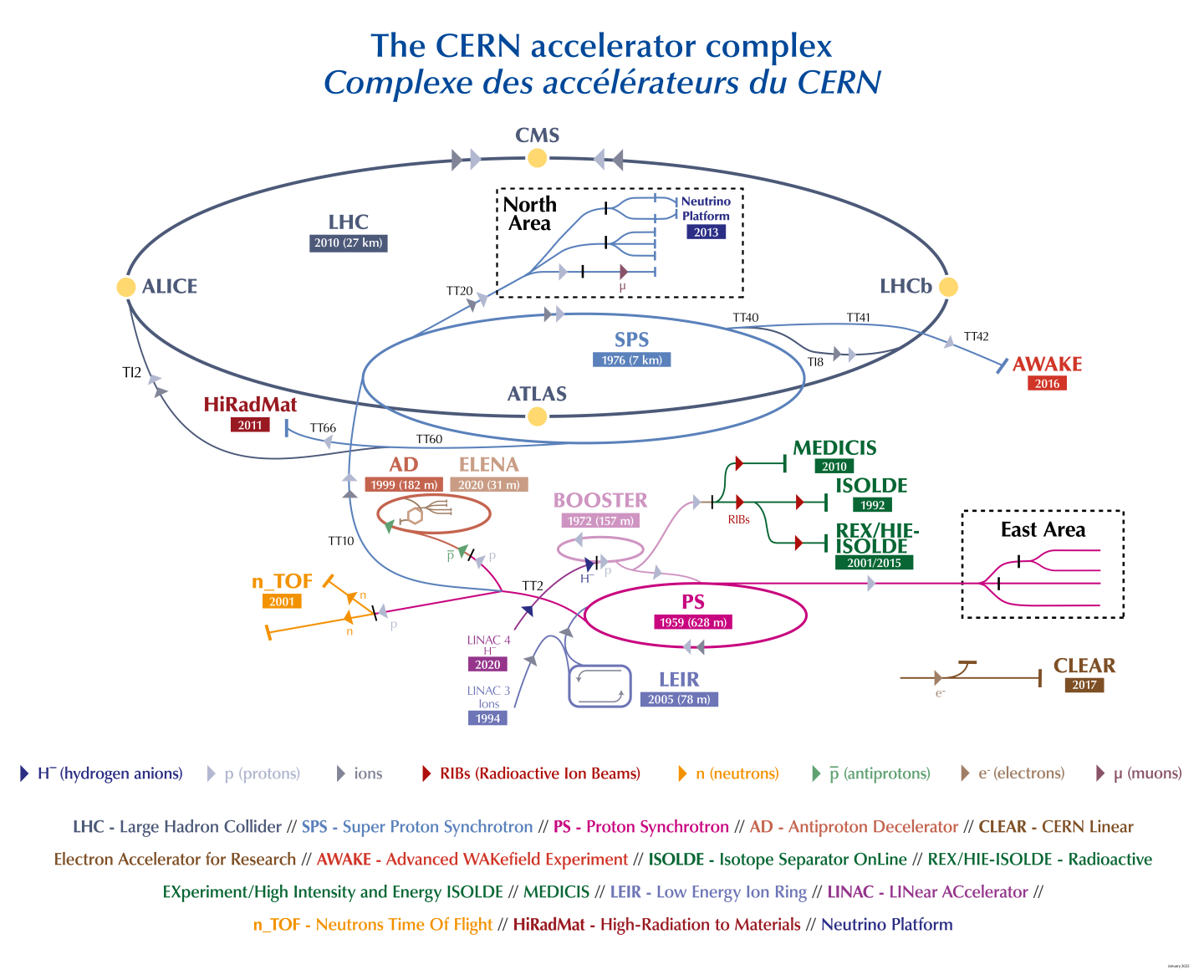
Part II: Simulation of Synchrotron Motion in the CERN Proton Synchrotron
The world's first synchrotron (1959), delivering beams to the LHC today!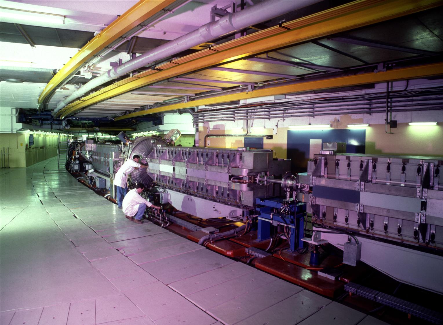
CERN PS Parameters
For reference, the CERN Proton Synchrotron (PS) parameters:
- has a circumference of 2π·100m
- takes protons from the PS Booster at a kinetic energy of 2 GeV (corresponding to $\gamma=3.13$)
- injects with 50 kV of RF voltage into stationary bucket, during magnetic ramp use 200 kV
- runs at harmonic $h=7$
- has a momentum compaction factor of $\alpha_c=0.027$
- typical acceleration rate of (up to) $\dot{B}=2$ T/s, the bending radius is $\rho=70.08$ m]
- extracts beams at 26 GeV (corresponding to $\gamma=28.7$)
Some convenience functions to compute the speed β and the relativistic Lorentz factor γ:
def beta(gamma):
    '''Speed β in units of c from relativistic Lorentz factor γ.'''
    return np.sqrt(1 - gamma**-2)

def gamma(p):
    '''Relativistic Lorentz factor γ from total momentum p.'''
    return np.sqrt(1 + (p / (mass * c))**2)
We gather all the machine parameters in a class named Machine to represent the CERN PS.
A Machine instance knows
- at which energy the synchronous particle (reference $\gamma_\text{ref}$,
gamma_ref, or alternatively the momentump0()) currently runs, - what the acceleration rate is in terms of the synchronous phase $\varphi_s$,
phi_s - how to compute the phase-slip factor $\eta$,
eta, for a particle at a certain momentum $p_0 + \Delta p$ - how to update the energy of the synchronous particle via
update_gamma_ref()when a turn has passed
charge = e
mass = m_p

class Machine(object):
    # units: SI, phi_s in rad:
    gamma_ref = 3.13 #fill me
    circumference = 2 * np.pi * 100 #fill me
    voltage = 50e3 #fill me
    harmonic = 7 #fill me
    alpha_c = 0.027 #fill me
    phi_s = 0.456 #fill me

    def __init__(self, gamma_ref=gamma_ref, circumference=circumference,
                 voltage=voltage, harmonic=harmonic,
                 alpha_c=alpha_c, phi_s=phi_s):
        '''Override default settings by giving explicit arguments.'''
        self.gamma_ref = gamma_ref
        self.circumference = circumference
        self.voltage = voltage
        self.harmonic = harmonic
        self.alpha_c = alpha_c
        self.phi_s = phi_s

    def eta(self, deltap):
        '''Phase-slip factor for a particle.'''
        p = self.p0() + deltap
        return self.alpha_c - gamma(p)**-2

    def p0(self):
        '''Momentum of synchronous particle.'''
        return self.gamma_ref * beta(self.gamma_ref) * mass * c

    def update_gamma_ref(self):
        '''Advance the energy of the synchronous particle
        according to the synchronous phase by one turn.
        '''
        deltap_per_turn = charge * self.voltage / (
            beta(self.gamma_ref) * c) * np.sin(self.phi_s)
        new_p0 = self.p0() + deltap_per_turn
        self.gamma_ref = gamma(new_p0)
Hamiltonian landscape in longitudinal plane
Now we define the kinetic and potential energy terms:
def T(deltap, machine):
    '''Kinetic energy term in Hamiltonian.'''
    return -0.5 * machine.eta(deltap) / machine.p0() * deltap**2

def U(z, machine, beta_=None):
    '''Potential energy term in Hamiltonian.
    If beta is not given, compute it from synchronous particle.
    '''
    m = machine
    if beta_ is None:
        beta_ = beta(gamma(m.p0()))
    ampl = charge * m.voltage / (beta_ * c * 2 * np.pi * m.harmonic)
    phi = m.phi_s - 2 * np.pi * m.harmonic / m.circumference * z
    # convenience: define z at unstable fixed point
    z_ufp = -m.circumference * (np.pi - 2 * m.phi_s) / (2 * np.pi * m.harmonic)
    # convenience: offset by potential value at unstable fixed point
    # such that unstable fixed point (and separatrix) have 0 potential energy
    return ampl * (-np.cos(phi) +
                   2 * np.pi * m.harmonic / m.circumference * (z - z_ufp) * np.sin(m.phi_s) +
                   -np.cos(m.phi_s))
...and the Hamiltonian function(al) itself:
def hamiltonian(z, deltap, machine):
    return T(deltap, machine) + U(z, machine, beta_=beta(gamma(machine.p0() + deltap)))
Some plotting helper functions:
from config import plot_hamiltonian, plot_rf_overview
Setting up the PS
The Machine instance will keep track of the reference energy during the tracking by calling update_gamma_ref() once per turn.
You can override the default PS parameters by supplying arguments to the Machine(...) instantiation, e.g. change the gamma_ref by m = Machine(gamma_ref=20) or the phi_s etc.
m = Machine(phi_s=0)
Let's plot the Hamiltonian landscape on phase space:
$\implies$ the closed area inside the blue separatrix is typically referred to as "RF bucket"!
plot_hamiltonian(m)

Exercises based on Hamiltonian
Change the settings of Machine (notably phi_s and gamma_ref) here to explore the consequences on the Hamiltonian landscape (and hence the predicted particle orbits).
- For $\varphi_s=0$, compare the stationary situation of the synchronous particle to a nonlinear pendulum:
- What is the meaning of a $\varphi_s=0,\pi$ synchronous phase offset in terms of the pendulum?
- What state of a pendulum does the stable fixed point, and the unstable fixed point, correspond to?
- What happens to the separatrix / rf bucket for a small change around $\varphi_s=0$? Use the
plot_rf_overviewfunction below to visualise the potential.
- For $\varphi_s=0$, what happens if you set an energy above transition? You will need to compute $\gamma_t=1/\sqrt{\alpha_c}$.
- Calculate the correct $\varphi_s$ to achieve the acceleration rate of $\dot{B}=2$ T/s. You may use the convenience functions below. What is the fractional increase in the reference momentum per turn, $(\delta p_0)_\text{turn}/p_0$? What happens to the separatrix?
plot_rf_overview(m);

To compute a synchronous phase $\varphi_s$, you may use these convenience functions to compute the $\arcsin$ on the interval of [-π/2,π/2] .
def deltap_per_turn(Bdot, rho, circumference, p0):
    Trev = circumference / (beta(gamma(p0)) * c)
    return Bdot * rho * charge * Trev
def compute_phi_s(deltap_per_turn, p0, voltage):
    '''Return *first* positive phase which matches the
    given Δp/turn on the interval [0, π/2].
    Do check whether you need to use π-φ_s for stability!
    '''
    return np.arcsin(
        deltap_per_turn * beta(gamma(p0)) * c / (charge * voltage)
    )
Compute the synchronous phase:
(NB: Remember you may likely want to find a synchronous phase on $\varphi_s\in[0,π]$ (why?)!)
Particle Tracking
As a reminder, the tracking equations for the longitudinal plane read:
$$\begin{cases}\, z_{n+1} &= z_n - \eta C \left(\cfrac{\Delta p}{p_0}\right)_n \\ (\Delta p)_{n+1} &= (\Delta p)_n + \cfrac{q V}{(\beta c)_n}\cdot\left(\sin\left(\varphi_s - \cfrac{2\pi}{C}\cdot hz_{n+1}\right) - \sin(\varphi_s)\right) \end{cases}$$
def track_one_turn(z_n, deltap_n, machine):
    m = machine
    # drift
    z_n1 = z_n - m.eta(deltap_n) * deltap_n / m.p0() * m.circumference
    # rf kick
    amplitude = charge * m.voltage / (beta(gamma(m.p0())) * c)
    phi = m.phi_s - m.harmonic * 2 * np.pi * z_n1 / m.circumference

    m.update_gamma_ref()
    deltap_n1 = deltap_n + amplitude * (np.sin(phi) - np.sin(m.phi_s))
    return z_n1, deltap_n1
Setting up the PS Machine for tracking:
(hint: hit both Shift+Tab keys inside the parentheses () below to get info about the possible arguments to Machine)
m = Machine(phi_s=0, gamma_ref=3.13) #, voltage=...)
Particle trajectories are tracked by their two longitudinal coordinates $(z, \Delta p)$. The initial values are stored in z_ini and deltap_ini as numpy.arrays. These should have N entries for $N$ particles.
(You may use numpy helper functions such as np.linspace or np.arange for convenient initialisation!)
n_turns = 500 # change me
deltap_ini = np.linspace(0, 0.01 * m.p0(), 20) # change me
z_ini = np.zeros_like(deltap_ini) # replace me

N = len(z_ini)
assert (N == len(deltap_ini))
To store the coordinate values during tracking, prepare some n_turns long 2D arrays with N entries per turn:
z = np.zeros((n_turns, N), dtype=np.float64)
deltap = np.zeros_like(z)

z[0] = z_ini
deltap[0] = deltap_ini
Record the evolution of energy $\gamma_\mathrm{ref}$ and also Hamiltonian values of particles during tracking:
gammas = np.zeros(n_turns, dtype=np.float64)
gammas[0] = m.gamma_ref

H_values = np.zeros_like(z)
H_values[0] = hamiltonian(z_ini, deltap_ini, m) / m.p0()
Tracking Loop
Let's go, here's the tracking loop over the number of turns n_turns!
for i_turn in range(1, n_turns):
    # track & record:
    z[i_turn], deltap[i_turn] = track_one_turn(z[i_turn - 1], deltap[i_turn - 1], m)
    # record:
    gammas[i_turn] = m.gamma_ref
    H_values[i_turn] = hamiltonian(z[i_turn], deltap[i_turn], m) / m.p0()
Change of energy during simulation
plt.plot(gammas)
plt.xlabel('Turns')
plt.ylabel('$\gamma_{ref}$')
Text(0, 0.5, '$\\gamma_{ref}$')

Phase space evolution during simulation
# plot_hamiltonian(m); # uncomment me

plt.scatter(z, deltap / m.p0(), marker='.', s=0.5)
plt.xlabel('$z$ [m]')
plt.ylabel('$\Delta p/p_0$')
Text(0, 0.5, '$\\Delta p/p_0$')

Evolution of Hamiltonian / energy value during simulation
plt.plot(H_values, c='C0');
plt.axhline(0, c='r', ls='--')
plt.xlabel('Turns')
plt.ylabel(r'$\mathcal{H}(z,\Delta p)\,/\,p_0$');

Overview of longitudinal phase space landscape
plot_rf_overview(m);
Exercises based on Tracking
Modify the machine parameters (and initial coordinates of particles) starting here to answer the following questions:
- For $\varphi_s=0$, can you identify which particles are stably focused inside the RF bucket, and which ones are unbound outside?
- For the correct $\varphi_s>0$, what happens to particles outside the RF bucket now?
- Do the Hamiltonian contours predict the tracked particle trajectories well?
- CERN PS accelerates protons from $\gamma=3.1$ up to $\gamma=27.7$. Is the transition energy crossed during acceleration? What does this mean for the setting of the synchronous phase $\varphi_s$ in the control room?
- What happens to phase focusing at the transition energy $\gamma=\gamma_\mathrm{t}$? Can you explain why? (Think of the phase slippage mechanism.)
Summary
- beam rigidity equation: $B\rho=p/|q|$
- synchrotron principle, $f_\text{rf}=h\cdot f_\text{rev}$ with harmonic $h\in\mathbb{N}$
- momentum compaction $\alpha_c$ and phase-slip factor $\eta=\gamma_t^{-2}-\gamma^{-2}$
- transition energy $\gamma_t$
- longitudinal particle tracking equations for synchrotrons
- ordinary differential equations and Hamiltonian for synchrotron motion
- synchrotron tune
Bonus Exercise: Realistic Beam Simulation
In the following, let us properly simulate the full acceleration ramp (including crossing transition) with a realistic bunch. It shall be Gaussian distributed and cover a small phase-space area, referred to as a bunch of "small emittance" (phase-space area)!
You as operator in the (simulation) control centre shall pay attention to ensure stable phase focusing (and therefore preserve the longitudinal emittance) throughout the acceleration!
$\implies$ Investigate the tracking results. Can you explain what happens? Think about what you need to change in the machine settings to achieve emittance preservation.
m = Machine(phi_s=0.456)#fill me)

assert m.phi_s > 0, "machine is not accelerating...?"
We initialise a Gaussian bunch distribution with very small rms bunch length $\sigma_z=1\,$m (is this small compared to the RF bucket length? Would the small-amplitude Hamiltonian approximation be expected to hold, accordingly?):
sigma_z = 1
The "matched" rms momentum spread $\sigma_{\Delta p}$:
(NB: a matched distribution is in equilibrium. $\sigma_{\Delta p}$ and $\sigma_z$ are linked to each other via equal Hamiltonian values $\mathcal{H}_0$, as they should both correspond to the same iso-Hamiltonian contour – that is the equilibrium condition.)
sigma_deltap = np.sqrt(
    2 * m.p0() / -m.eta(0) *
    charge * m.voltage * np.pi * m.harmonic / (beta(gamma(m.p0())) * c * m.circumference**2)
) * sigma_z
N = 1000
np.random.seed(12345)

z = np.random.normal(loc=0, scale=sigma_z, size=N)
deltap = np.random.normal(loc=0, scale=sigma_deltap, size=N)
plot_hamiltonian(m)
plt.scatter(z, deltap / m.p0(), marker='.', s=1);

Compute Duration of Ramp
$(\Delta\gamma)_\mathrm{turn} = \cfrac{\Delta E_\mathrm{tot}}{m_0c^2} = \cfrac{qV\sin(\varphi_s)}{m_0c^2}$
such that accelerating from $\gamma_\mathrm{ref}=3.1$ to $\gamma_\mathrm{ref}=27.7$ takes as many turns as
$n_\mathrm{turns}=\cfrac{27.7-3.1}{(\Delta\gamma)_\mathrm{turn}}$
dgamma_per_turn = charge * m.voltage * np.sin(m.phi_s) / (mass * c**2)
n_turns = int(np.ceil((27.7 - 3.13) / dgamma_per_turn))
n_turns
1047022
Record longitudinal emittance during tracking:
from config import emittance
epsn_z = np.zeros(n_turns, dtype=np.float64)

epsn_z[0] = emittance(z, deltap)
Let's go tracking! ($\approx 1\,$min total time)
for i_turn in trange(1, n_turns):
    z, deltap = track_one_turn(z, deltap, m)

    epsn_z[i_turn] = emittance(z, deltap)
0%| | 0/1047021 [00:00<?, ?it/s]
Have we reached the extraction energy of $\gamma=27.7$?
m.gamma_ref
np.float64(27.699981145999953)
How did we do?
Check that we properly conserved a constant rms emittance:
plt.plot(np.arange(n_turns) / 100000, epsn_z / e)

plt.xlabel('Turns [100k]')
plt.ylabel('$\epsilon_z$ [eV.s]');

$\implies$ use the following phase-space plot besides the plotting functions plot_hamiltonian and plot_rf_overview above as diagnostics. You can stop the tracking after a certain turn to investigate, e.g. by changing the value of n_turns inside the trange counter in the for loop.
plot_hamiltonian(m);
plt.scatter(z % 600, deltap / m.p0(), marker='.', s=1);

If the progress bar by tqdm (trange) in this document does not work, run this:
!jupyter nbextension enable --py widgetsnbextension
Enabling notebook extension jupyter-js-widgets/extension...
      - Validating: OK