S35 Accelerator & Detector Physics
Accelerator Physics by Professor Adrian Oeftiger
Lecture 6: Off-momentum Effects, Synchrotron Radiation
Run this notebook online!
Interact and run this jupyter notebook online:
Also find this lecture rendered as HTML slides on github $\nearrow$ along with the source repository $\nearrow$.
Run this first!
Imports and modules:
from config import (np, plt, sys, Madx, interp1d, PyNAFF,
                    pysixtrack, elements,
                    M_drift, M_dip_x, M_dip_y,
                    M_quad_x, M_quad_y,
                    track, track_sext_4D)
%matplotlib inline
Refresher!
- Hill Differential Equation & Floquet Theory
- Twiss Parametrisation and Optics
- The FODO Cell
Today!
- Off-momentum Particles: Dispersion & Chromaticity
- Synchrotron Radiation
Part I: Off-momentum Particles, Dispersion & Chromaticity
Off-momentum Trajectory
Particles with a momentum $p\neq p_0$ different from reference momentum $p_0$ are bent by magnetic fields $B$ on a different bending radius $\rho$:
$$B\rho=\cfrac{p}{|q|}$$
In particular, higher-momentum particles are bent less, and their off-momentum trajectory encompasses two major effects:
- Dispersion (dipole magnets, change of closed orbit)
- Chromaticity (quadrupole magnets, change of focusing)
image by Y. Hao
Dispersion
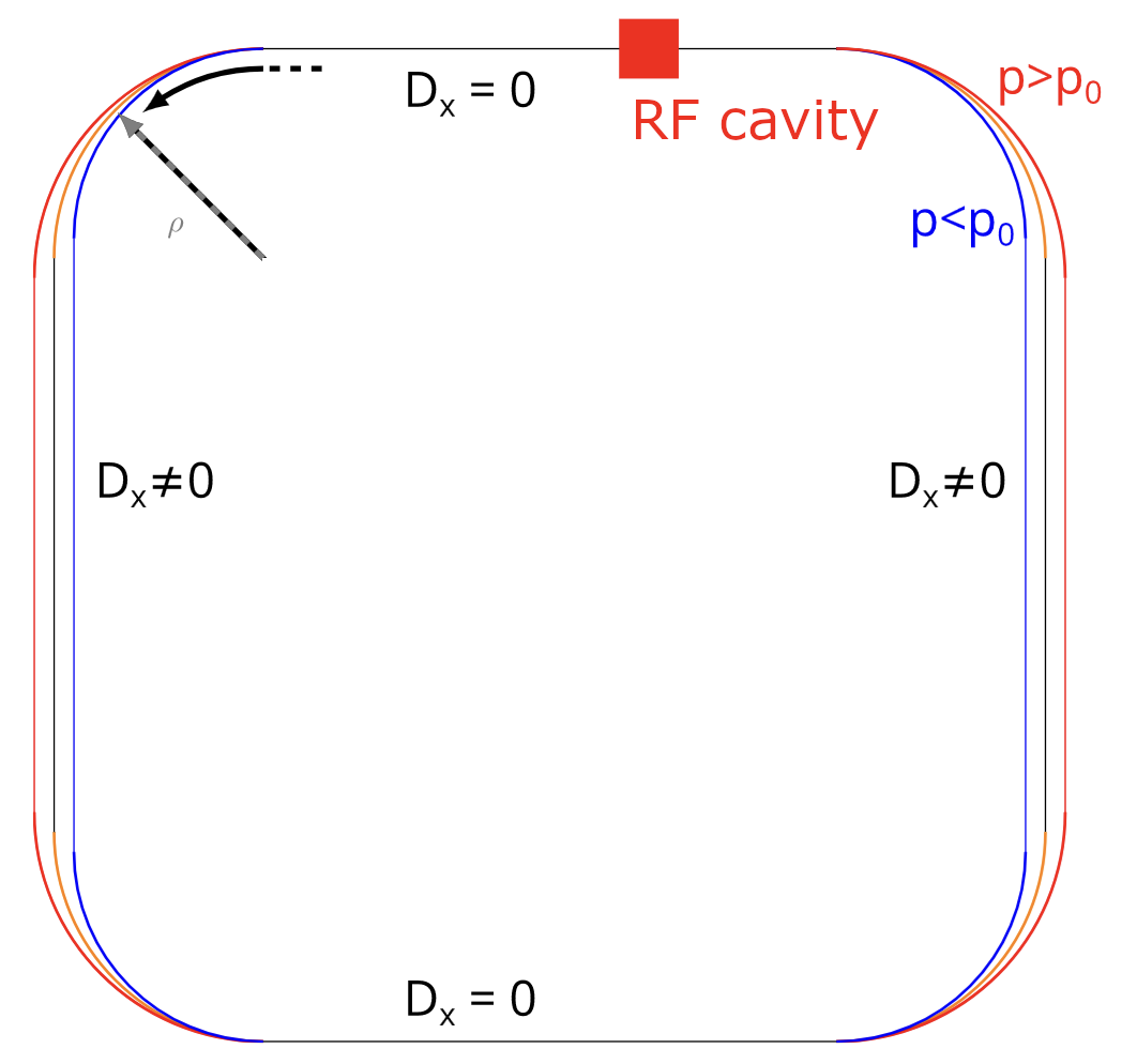
Since dipole magnets define the reference orbit (cf. Frenet-Serret coordinate system), off-momentum particles will experience a different "dispersive" closed orbit – dipoles are said to "generate" dispersion.
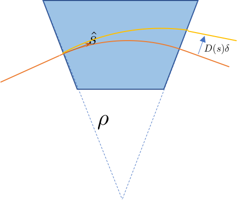
The dispersion function $D(s)$ describes the local equilibrium offset from the reference closed orbit due to a momentum deviation $\delta=\Delta p/p_0$ with respect to the synchronous reference particle:
$$x(s)=\underbrace{x_\beta}\limits_{\mathop{=}\sqrt{2J_x\beta_x(s)}\cos(\psi_x(s))} + x_\text{disp}\qquad\text{with}\qquad x_\text{disp}(s) = D_x(s) \cdot \delta$$
$D_x(s)$ hence represents the (horizontal) closed orbit for a particle with $\delta=1$, i.e. twice the reference momentum.
image by A. Lasheen / JUAS
Simulation 1: Computing the Dispersion Function of a FODO cell
For illustration, we use again the LHC FODO cell:
madx = Madx(stdout=sys.stdout)

madx.input('''
k1l_f := 0.008 * 3.3;  // inverse focal length qf
k1l_d := -0.008 * 3.3; // inverse focal length qd
theta := 0;            // in LHC: 2 * pi / 1232;

qf2: quadrupole, l = 3.3 / 2, k1 := k1l_f / 3.3; // half a focusing quad
qd:  quadrupole, l = 3.3,     k1 := k1l_d / 3.3;
dip: sbend, l = 14.3, angle := theta;

fodo: sequence, l = 110;
qf2, at = 3.3 / 4;
dip, at = 12;
dip, at = 2 * 110 / 8;
dip, at = 110 / 2 - 12;
qd, at = 110 / 2;
dip, at = 110 / 2 + 12;
dip, at = 6 * 110 / 8;
dip, at = 110 - 12;
qf2, at = 110 - 3.3 / 4;
endsequence;
''');

madx.command.beam(particle='proton', energy=7e3) # energy is in GeV!
madx.use(sequence='fodo')

# output the Twiss parameters every 1m
madx.command.select(flag="interpolate", sequence="fodo", step=1);

twiss = madx.twiss();
qx_fodo = twiss.summary['q1']
qpx_fodo = twiss.summary['dq1'] # multiplied by beta~1
  ++++++++++++++++++++++++++++++++++++++++++++
  +     MAD-X 5.09.03  (64 bit, Darwin)      +
  + Support: mad@cern.ch, http://cern.ch/mad +
  + Release   date: 2024.04.25               +
  + Execution date: 2026.05.08 11:22:59      +
  ++++++++++++++++++++++++++++++++++++++++++++
enter Twiss module

iteration:   1 error:   0.000000E+00 deltap:   0.000000E+00
orbit:   0.000000E+00  0.000000E+00  0.000000E+00  0.000000E+00  0.000000E+00  0.000000E+00

++++++ table: summ

            length             orbit5               alfa            gammatr
               110                 -0                  0                  0

                q1                dq1            betxmax              dxmax
      0.2518947018      -0.3220961047        186.9084848                  0

             dxrms             xcomax             xcorms                 q2
                 0                  0                  0       0.2518947018

               dq2            betymax              dymax              dyrms
     -0.3220961047        186.4581481                  0                  0

            ycomax             ycorms             deltap            synch_1
                 0                  0                  0                  0

           synch_2            synch_3            synch_4            synch_5
                 0                  0                  0                  0

           synch_6            synch_8             nflips              dqmin
                 0                  0                  0                  0

       dqmin_phase
                 0
madx.input('value, beam->beta;')
beam->beta = 0.999999991 ;
True
We "switch" on the dipole magnets by defining a non-zero bending angle:
madx.input('theta := 2 * pi / 1232;');
++++++ info: theta redefined
Let us recompute the optics functions, as this time also the dispersion function will assume finite values ($\leadsto$ why?):
twiss = madx.twiss();
enter Twiss module

iteration:   1 error:   0.000000E+00 deltap:   0.000000E+00
orbit:   0.000000E+00  0.000000E+00  0.000000E+00  0.000000E+00  0.000000E+00  0.000000E+00

++++++ table: summ

            length             orbit5               alfa            gammatr
               110                 -0    0.0004388874913        47.73351305

                q1                dq1            betxmax              dxmax
      0.2519723158      -0.3218296078        186.8781443        2.249453549

             dxrms             xcomax             xcorms                 q2
       1.634089545                  0                  0       0.2518947018

               dq2            betymax              dymax              dyrms
     -0.3218849941        186.4581481                  0                  0

            ycomax             ycorms             deltap            synch_1
                 0                  0                  0                  0

           synch_2            synch_3            synch_4            synch_5
                 0                  0                  0                  0

           synch_6            synch_8             nflips              dqmin
                 0                  0                  0                  0

       dqmin_phase
                 0
Given that $D=\cfrac{x}{\delta}$ for the equilibrium orbit at a momentum deviation $\delta$, the dispersion function $D(s)$ satisfies the inhomogeneous Hill differential equation
$$D'' + \left(\frac{1}{\rho_0(s)} + k(s)\right)\cdot D = \frac{1}{\rho_0(s)}$$
plt.plot(twiss['s'], twiss['dx'] * 0.999999991) # multiplied by beta~1
plt.xlabel('$s$ [m]')
plt.ylabel('$D_x(s)$ [m]');

$\implies$ Dispersion function $D(s)$ is focused by the quadrupoles, analogous to the horizontal $\beta_x(s)$-function!
$\leadsto$ Verify that the dispersion is generated by the dipole magnets! (What does this mean?) How does the dispersion function $D(s)$ look like when the dipole fields are switched off?
Simulation 2: Dispersion Effect in Tracking
To illustrate the dispersion effect, we use the thin-lens tracking code PySixTrack (like our thin-lens betatron matrices but for 6D, i.e. including the momentum deviation $\delta$)!
We define a drift of $5\,$m length and a dipole with a bending angle of $0.1\,$rad:
drift = elements.DriftExact(5)
dipole = elements.Multipole(knl=[0.1], hxl=0.1)
Initialise two particles, both at $x=0.04\,$m but only one at a momentum deviation of $\delta=10^{-3}$:
part0 = pysixtrack.Particles(x=0, delta=0)
part1 = pysixtrack.Particles(x=0, delta=0.001)
Track through the drift, then the dipole and again the drift:
rec_x0 = [part0.x]
rec_x1 = [part1.x]

drift.track(part0)
drift.track(part1)

rec_x0 += [part0.x]
rec_x1 += [part1.x]

dipole.track(part0)
dipole.track(part1)

rec_x0 += [part0.x]
rec_x1 += [part1.x]

drift.track(part0)
drift.track(part1)

rec_x0 += [part0.x]
rec_x1 += [part1.x]
plt.plot([0, 5, 5, 10], rec_x0, label='$\delta=0$')
plt.plot([0, 5, 5, 10], rec_x1, label='$\delta=10^{-3}$')

plt.xlabel('$s$ [m]')
plt.ylabel('$x$ [m]')
plt.legend();

$\leadsto$ Please explain what happens here and why.
Chromaticity
Chromaticity describes the change of focusing for off-momentum particles at $p=p_0(1+\delta)$.
The chromatic aberration of a quadrupole focusing lens with gradient $\frac{\partial B_y}{\partial x}$ yields:
$$k \equiv \cfrac{1}{B\rho}\cfrac{\partial B_y}{\partial x} \propto \cfrac{1}{p}\implies k(\delta)=\cfrac{k}{1+\delta}$$
Therefore, quadrupoles focus less for higher-momentum particles $\delta>0$ and thus the tune $Q$ decreases. The chromaticity of an accelerator is defined as
$$Q'=\frac{dQ}{d\delta}$$
The natural chromaticity of a (linear) magnetic lattice is typically negative.
Simulation 3: Chromaticity Effect in Tracking
Let us illustrate by tracking particles in PySixTrack again. We define a quadrupole with an integrated focusing strength of $k\cdot L=0.3\,$m${}^{-1}$:
quad = elements.Multipole(knl=[0, 0.3])
$\leadsto$ What is the expected focal length $f=\cfrac{1}{k\cdot L}$?
Initialise two sets of particles with the same distribution in $x$, one of which features a momentum deviation of $\delta=0.1$ (!):
$\leadsto$ What is the expected focal length change $\Delta f(\delta)$ for these $\delta=0.1$ particles?
npart = 11
x_dist = np.linspace(-0.05, 0.05, npart)
part0 = pysixtrack.Particles(x=x_dist.copy(), delta=0)
part1 = pysixtrack.Particles(x=x_dist.copy(), delta=0.1)
Track through the $5\,$m drift, then through the quadrupole and again through the same drift:
rec_x0 = [part0.x.copy()]
rec_x1 = [part1.x.copy()]

drift.track(part0)
drift.track(part1)

rec_x0 += [part0.x.copy()]
rec_x1 += [part1.x.copy()]

quad.track(part0)
quad.track(part1)

rec_x0 += [part0.x.copy()]
rec_x1 += [part1.x.copy()]

drift.track(part0)
drift.track(part1)

rec_x0 += [part0.x.copy()]
rec_x1 += [part1.x.copy()]
for i in range(npart):
    l0, = plt.plot([0, 5, 5, 10], np.array(rec_x0)[:, i], c='C0', lw=1)
    l1, = plt.plot([0, 5, 5, 10], np.array(rec_x1)[:, i], c='C1', lw=1)

plt.xlabel('$s$ [m]')
plt.ylabel('$x$ [m]')
plt.legend([l0, l1], ['$\delta=0$', '$\delta=0.1$']);

$\implies$ We observe less focusing for $\delta>0$ particles $\implies$ less phase advance in quasi-harmonic oscillation $\implies$ negative tune shift!
Natural Chromaticity of a FODO Cell
Natural chromaticity of a FODO cell with phase advance $\Phi_\text{FODO}$ can be derived via thin-lens approximation (lecture 4):
$$Q'_\text{FODO} = -\frac{1}{\pi}\tan\left(\frac{\Phi_\text{FODO}}{2}\right)$$
Natural chromaticity is always negative ($\leadsto$ why?).
Simulation 4: Chromatic Detuning in a FODO Cell from Tracking
Let us track with PySixTrack through the LHC FODO cell for a distribution of particles with momentum spread and observe the chromatic tune shift.
We first define the same FODO cell as in MAD-X before (just in thin-lens approximation and without dipoles):
kL = 0.008 * 3.3

qf2_fodo = elements.Multipole(knl=[0, kL / 2.])
qd_fodo = elements.Multipole(knl=[0, -kL])
drift_fodo = elements.DriftExact(110 / 2.)

fodo = [qf2_fodo, drift_fodo, qd_fodo, drift_fodo, qf2_fodo]
We initialise a distribution of npart macro-particles, with a momentum spread between $\delta\in[-10^{-3},10^{-3}]$ at a fixed initial horizontal position of $x=0.04\,$m:
npart = 21
x_ini = 0.04
delta = np.linspace(-0.001, 0.001, npart)

particles = pysixtrack.Particles(x=x_ini, delta=delta)
We will record the $x$ position after each FODO cell for each particle:
ncells = 1024

rec_x = np.zeros((ncells, npart), dtype=float)
rec_x[0] = particles.x
Let's go for the tracking:
for i in range(1, ncells):
    for el in fodo:
        el.track(particles)
    rec_x[i] = particles.x
Comparing two particles with same initial $x$ but different $\delta$, we already see the different phase advance in the recorded horizontal motion:
plt.plot(rec_x[:, npart//2 + 1], lw=2, label='$\delta=0$')
plt.plot(rec_x[:, 0], lw=2, label='$\delta=-0.001$')

plt.xlabel('number of FODO cells')
plt.ylabel('$x$ [m]')
plt.legend(bbox_to_anchor=(1.05, 1));

Let's evaluate the tune of each particle using the NAFF algorithm:
Qx_delta = np.zeros(npart, dtype=float)

for i in range(npart):
    Qx_delta[i] = PyNAFF.naff(rec_x[:, i], turns=ncells, nterms=1)[0, 1]
The tune of the $\delta=0$ particle should be the tune of the reference particle in this linear lattice:
Qx_delta[npart//2 + 1]
np.float64(0.2585892190147644)
qx_fodo
0.2518947018
plt.plot(1e3 * delta, Qx_delta)

plt.xlabel('$\delta$ [$10^{-3}$]')
plt.ylabel('$Q_x$');

$\implies$ The tune changes with the momentum, as anticipated! The slope of this line is the first-order chromaticity $Q'_x$!
The numpy function polyfit is useful for a quick linear regression, the output is $(a,b)$ for $y=a\cdot x + b$:
np.polyfit(delta, Qx_delta, 1)
array([-0.3360318 , 0.25862306])
The slope and thus the chromaticity of the LHC FODO cell is approximately $Q'_x=-0.3$, measured via particle tracking.
Comparison
The analytic formula $Q'_\text{FODO} = -\frac{1}{\pi}\tan\left(\frac{\Phi_\text{FODO}}{2}\right)$ gives:
-1 / np.pi * np.tan(2 * np.pi * qx_fodo / 2)
np.float64(-0.32212202611662033)
MAD-X would have given us this value, too, we evaluated it as twiss.summary['dq1'] * beta (where beta is the speed of the particles):
qpx_fodo
-0.3220961047
Bonus: Chromaticity Correction with Sextupoles
On average over many turns (during which $\delta$ remains more or less constant – remember synchrotron motion is much slower than tranverse betatron motion), the horizontal position of the particles corresponds to their dispersive closed orbit:
$$\langle x \rangle = \langle x_\beta + x_\text{disp}\rangle = \langle \sqrt{2J\beta_x}\underbrace{\cos(\psi_x+\psi_{x0}) }\limits_{\langle\cos\rangle\mathop{=}0}\rangle + \langle D\cdot \delta\rangle = D\cdot \delta$$
Sextupole magnets provide a means to correct for chromaticity in a location where $D(s)\neq 0$ such that particles are on average sorted by momentum $\delta$.
Bonus Simulation 5: Chromaticity Correction in a FODO Cell
For demonstration, we add sextupoles to the FODO lattice in MAD-X and compute their necessary strength.
Make sure that dipoles are switched on, the dipole angle theta should be non-zero:
madx.input('value, theta;')
theta = 0.005099988074 ;
True
(Otherwise re-run the notebook in order, you need the line madx.input('theta := 2 * pi / 1232;'))
We add two sextupole magnets, one next to each quadrupole:
madx.input('sext1: sextupole, l = 1, k2 := k2sext1;')
madx.input('sext2: sextupole, l = 1, k2 := k2sext2;')
madx.command.seqedit(sequence='fodo')
madx.command.install(element='sext1', at=3.3/2 + 1)
madx.command.install(element='sext2', at=110/2 + 3.3/2 + 1)
madx.command.endedit()
++++++ info: seqedit - number of elements installed:  2
++++++ info: seqedit - number of elements moved:      0
++++++ info: seqedit - number of elements removed:    0
++++++ info: seqedit - number of elements replaced:   0
True
madx.use('fodo')
madx.input(
'''match, sequence = fodo;
global, sequence = fodo, dq1 = {Qpx}, dq2 = {Qpy};
vary, name = k2sext1, step = 0.0001;
vary, name = k2sext2, step = 0.0001;
lmdif, tolerance = 1e-12;
endmatch;
'''.format(Qpx=0, Qpy=0))
START MATCHING

number of sequences: 1
sequence name: fodo
number of variables:    2
user given constraints: 2
total constraints:      2

START LMDIF:

Initial Penalty Function =   0.20718425E+00


call:       4   Penalty function =   0.11711009E-26
 ++++++++++ LMDIF ended: converged successfully
call:       4   Penalty function =   0.11711009E-26

MATCH SUMMARY

Node_Name                  Constraint   Type  Target Value       Final Value        Penalty
--------------------------------------------------------------------------------------------------
Global constraint:         dq1          4     0.00000000E+00     2.20777692E-14     4.87427893E-28
Global constraint:         dq2          4     0.00000000E+00    -2.61471410E-14     6.83672981E-28


Final Penalty Function =   1.17110087e-27


Variable                 Final Value  Initial Value Lower Limit  Upper Limit
--------------------------------------------------------------------------------
k2sext1                   1.27667e-02  0.00000e+00 -1.00000e+20  1.00000e+20
k2sext2                  -2.53671e-02  0.00000e+00 -1.00000e+20  1.00000e+20

END MATCH SUMMARY

VARIABLE "TAR" SET TO   1.17110087e-27
True
$\implies$ The iterative algorithm in MAD-X has found suitable values of the sextupole strengths k2sext1 and k2sext2 such that the target chromaticity has been corrected to 0.
twiss = madx.twiss();

twiss.summary.dq1 # this is the chromaticity
enter Twiss module

iteration:   1 error:   0.000000E+00 deltap:   0.000000E+00
orbit:   0.000000E+00  0.000000E+00  0.000000E+00  0.000000E+00  0.000000E+00  0.000000E+00

++++++ table: summ

            length             orbit5               alfa            gammatr
               110                 -0    0.0004388874913        47.73351305

                q1                dq1            betxmax              dxmax
      0.2519723158     2.20777692e-14        186.8781443        2.249453549

             dxrms             xcomax             xcorms                 q2
       1.634424445                  0                  0       0.2518947018

               dq2            betymax              dymax              dyrms
  -2.614714098e-14        186.4581481                  0                  0

            ycomax             ycorms             deltap            synch_1
                 0                  0                  0                  0

           synch_2            synch_3            synch_4            synch_5
                 0                  0                  0                  0

           synch_6            synch_8             nflips              dqmin
                 0                  0                  0                  0

       dqmin_phase
                 0
2.20777692e-14
$\implies$ The chromaticity from the MAD-X optics computation has really become (numerically) zero!
We return to the PySixTrack tracking: after adding sextupoles of these strengths and the dipole magnets, we should be able to see the change via evaluating the chromaticity via NAFF from tracking data again!
As a short cut, we make the MAD-X lattice "thin" (apply thin-lens approximation) and transfer the lattice with dipoles and sextupoles to PySixTrack:
assert madx.command.select(
    flag='MAKETHIN',
    class_='quadrupole',
    slice_=1,
)

assert madx.command.select(
    flag='MAKETHIN',
    class_='sextupole',
    slice_=1,
)

assert madx.command.select(
    flag='MAKETHIN',
    class_='sbend',
    slice_=1,
)

madx.command.makethin(
    makedipedge=False,
    style='simple',
    sequence='fodo',
)

fodo_sext = pysixtrack.Line.from_madx_sequence(madx.sequence.fodo)
makethin: style chosen : simple
makethin: slicing sequence : fodo
#for el in fodo_sext.elements:
#    print (el)
Going on with particle tracking:
# define initial particle distribution & prepare recording array
particles = pysixtrack.Particles(x=x_ini, delta=delta)

rec_x = np.zeros((ncells, npart), dtype=float)
rec_x[0] = particles.x
# tracking!
for i in range(1, ncells):
    fodo_sext.track(particles)
    rec_x[i] = particles.x
plt.plot(rec_x[:, npart//2 + 1], lw=2, label='$\delta=0$')
plt.plot(rec_x[:, 0], lw=2, label='$\delta=-0.001$')

plt.xlabel('number of FODO cells')
plt.ylabel('$x$ [m]')
plt.legend(bbox_to_anchor=(1.05, 1));

# evaluate tunes via NAFF
Qx_delta = np.zeros(npart, dtype=float)

for i in range(npart):
    Qx_delta[i] = PyNAFF.naff(rec_x[:, i], turns=ncells, nterms=1)[0, 1]
plt.plot(1e3 * delta, Qx_delta)

plt.xlabel('$\delta$ [$10^{-3}$]')
plt.ylabel('$Q_x$');

The fit for the now much flatter slope of the tune change with $\delta$ gives:
np.polyfit(delta, Qx_delta, 1)
array([-0.01098794, 0.25440583])
$\implies$ $Q'_x=-0.01$ is nearly zero, i.e. the chromaticity correction scheme works! (The remainders are due to the thin-lens approximation!)
Hint: we have used 2 sextupoles as 2 degrees of freedom to correct both the horizontal and the vertical chromaticity to zero. One could use only one sextupole degree of freedom, but then only one of the transverse planes can be corrected to $Q'=0$, the other one likely increases!
Part II: Synchrotron Radiation
Synchrotron Radiation
Synchrotron light: electromagnetic radiation emitted by charged particles when accelerated in external magnetic field.
$\implies$ Could be from any source (e.g. astrophysical), but is generally thought of as coming from a man-made relativistic beam of electrons.
$\implies$ Synchrotron radiation sources:
- high-brightness photon beams
- tunability of photon spectrum
- pulsed time structure
image by T. Uruga
Emitted power per radiating particle
Moving charged particle source $=$ time-varying charge and current density $\implies$ Maxwell equations and wave equation to find EM fields $\implies$ frequency distribution of radiation and critical frequency $\omega_c$ (median of spectrum)
$$\omega_c=\cfrac{3}{2}\cfrac{c}{\rho}\gamma^3$$
$\implies$ Integrating over spectrum yields total radiated power
$$P_\gamma = \cfrac{e^2c}{6\pi\epsilon_0}\cfrac{\gamma^4}{\rho^2}$$
- decreasing bending radius $\rho$ (more bending!) increases critical frequency and power
- mass of particles enters via $\gamma=E_\text{tot}/m_0c^2$ $\implies$ $P_\gamma\propto 1/m_0^4$
(electrons radiate much more than protons!)
image by I. Martin / Diamond
Two Types of Sources
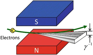
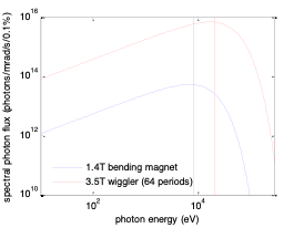
Bending magnet (dipole) vs. insertion device (wiggler / undulator):
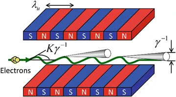
images by T. Uruga
Advantage of insertion devices:
- alternating permanent magnets force electrons onto sinusoidal trajectories
- extremely focused, i.e. ultra-bright photon beams
- wigglers: stronger deflection, broad spectrum
- undulators: weaker deflection, waves interfere constructively, almost mono-chromatic coherent synchrotron light
Synchrotron Radiation Facilities
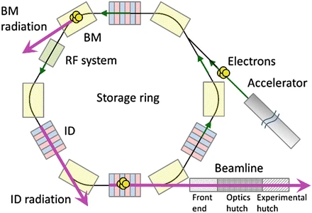
image by T. Uruga
Two categories of synchrotron radiation facilities:
- Storage rings
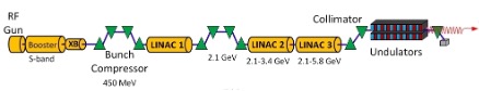
- Linac-based sources
$\implies$ Free Electron Lasers:
photon beam intensity $I\propto N_e^2$ instead of $I\propto N_e$ for conventional sources
Future Circular lepton Collider FCC-ee
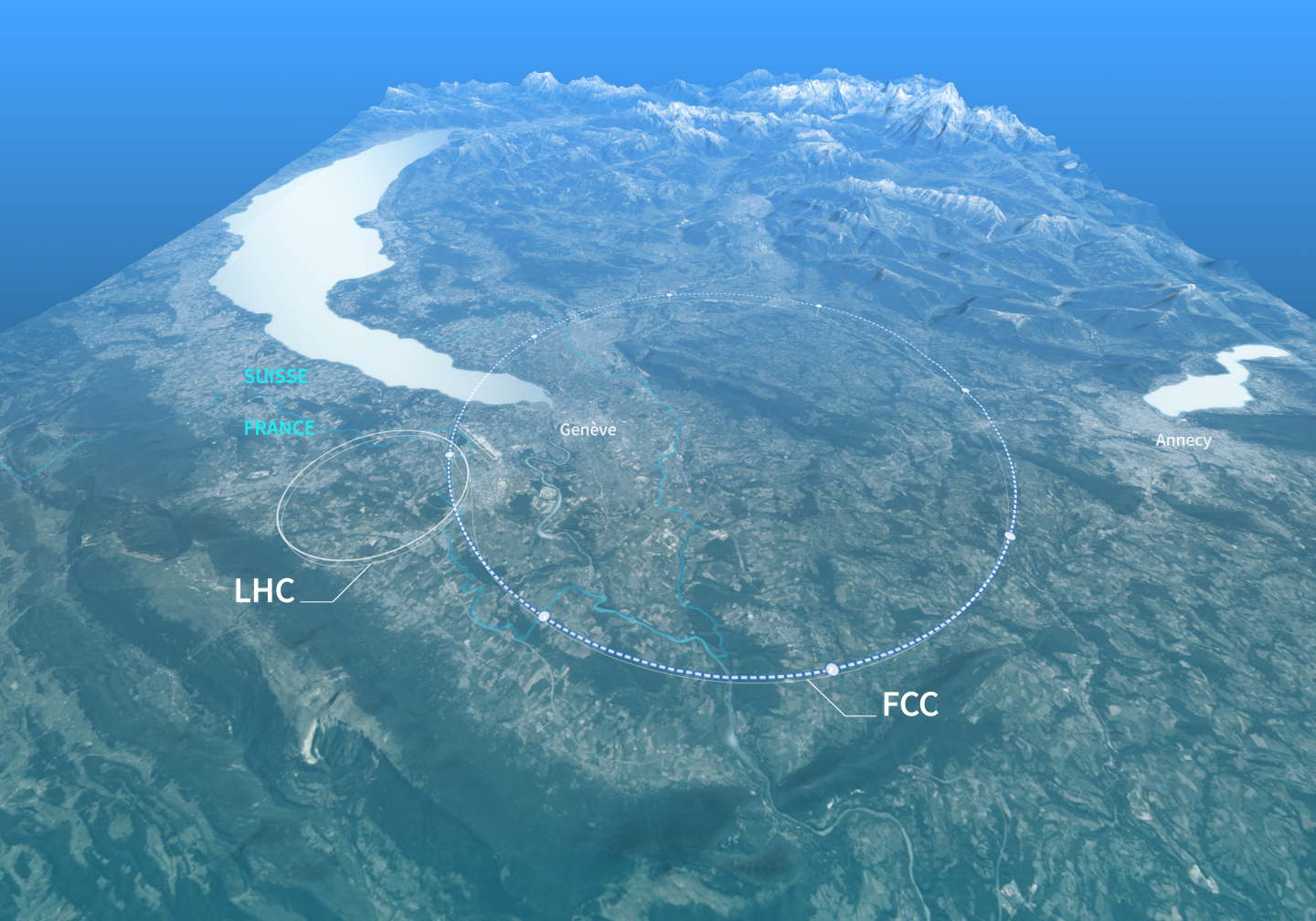
images by CERN
On the high-energy physics front:
next-generation facility for high-precision experiments
$\implies$ Higgs factory to study properties of Higgs
(discovered at LHC in 2012)
Collide leptons (electrons and positrons) for clean initial state during collision, much smaller background compared to proton colliders $\implies$ precision measurements!
European Particle Physics Strategy Update 2026: consider 91 km long FCC-ee proposal as top priority
$\implies$ Key issue of circular high-energy lepton colliders: synchrotron radiation (50 MW / beam!)
Synchrotron Radiation for Beam Size Detectors
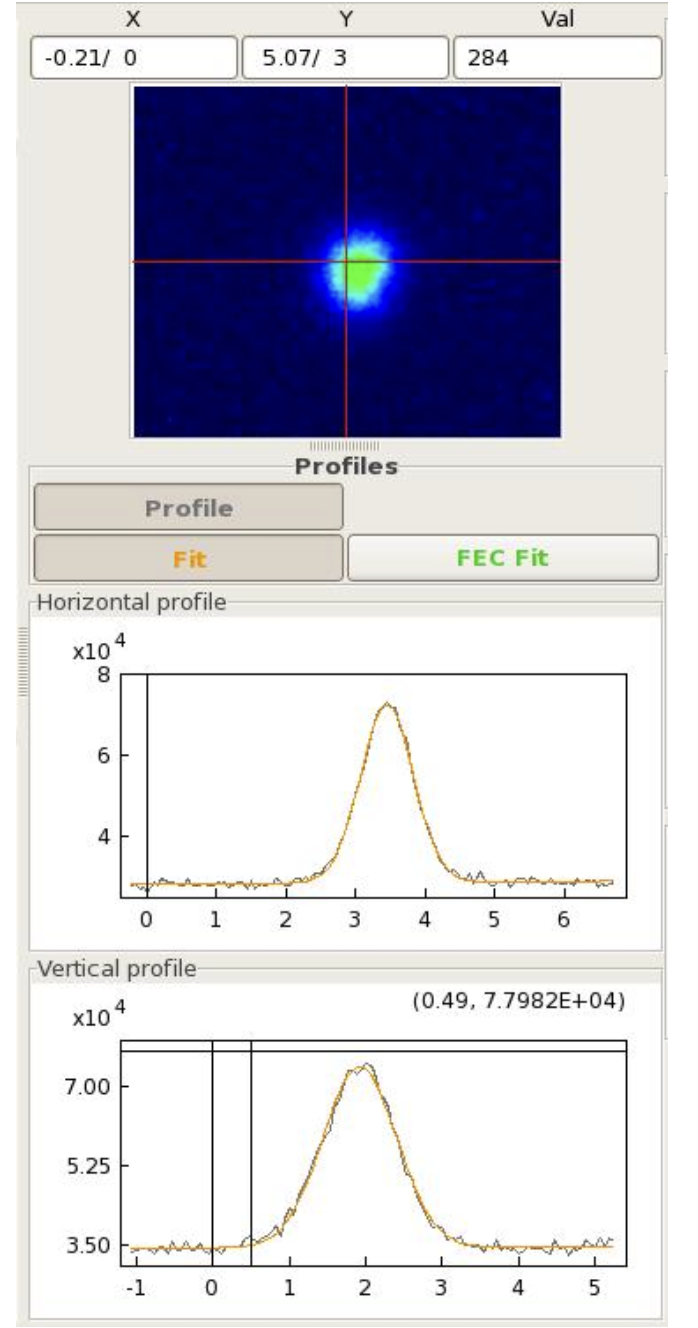
LHC employs BSRT system: Beam Synchrotron Radiation Telescope
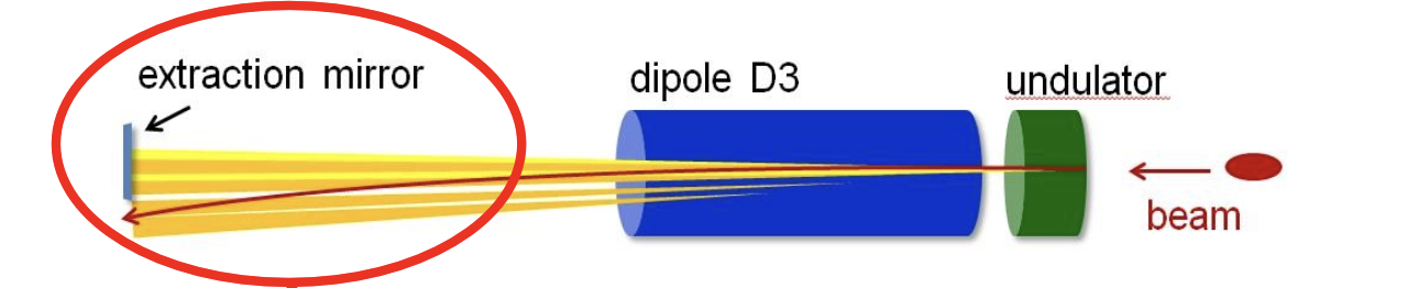
images by F. Caspers
$\implies$ At TeV level, protons do provide enough synchrotron radiation to be "seen"!
Summary
- Optical / Twiss functions and Dispersion of a FODO cell
- Dipoles generate & quadrupoles focuse dispersion function
- Quadrupole focal length depends on momentum, tune change, chromaticity
- Synchrotron radiation from accelerating/bending charged particles
- Light sources vs. HEP
TT26 Survey
Thank you very much!