S35 Accelerator & Detector Physics
Accelerator Physics by Professor Adrian Oeftiger
Lecture 5: Hill Equation and Stable Beam Transport
Run this notebook online!
Interact and run this jupyter notebook online:
Also find this lecture rendered as HTML slides on github $\nearrow$ along with the source repository $\nearrow$.
Run this first!
Imports and modules:
from config import (np, plt, sys, Madx, interp1d, PyNAFF,
                    M_drift, M_dip_x, M_dip_y,
                    M_quad_x, M_quad_y,
                    track, track_sext_4D, plot_twiss)
%matplotlib inline
Refresher!
- magnetic fields for bending particles in the transverse plane (vs. electric fields)
- multipole representation (normal and skew coefficients $b_n,a_n$)
- dipole, quadrupole, sextupole magnetic fields
- equation of motion in magnetic fields (after paraxial approximation)
- Hill differential equation
- betatron matrices for transport (solution to e.o.m.)
- drifts: divergence
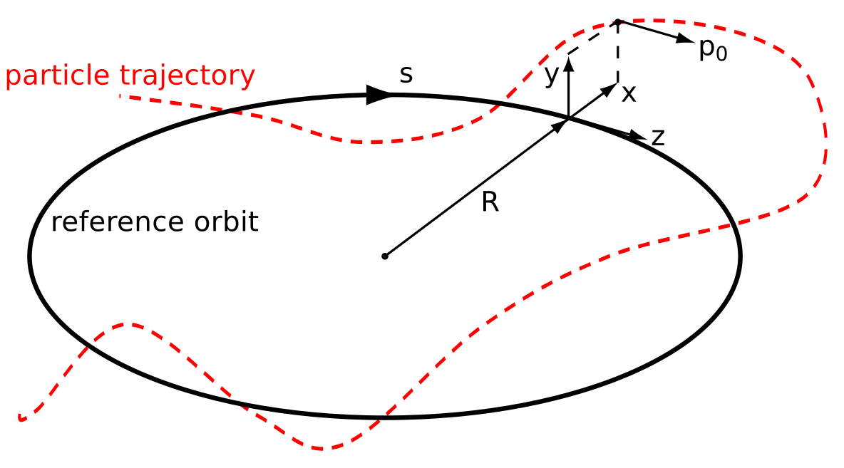
- dipoles: bending included in Frenet-Serret coordinate system, (weak) geometric focusing
- quadrupoles: focus in one plane while defocusing in the other
- FODO cells: alternating-gradient configuration stabilising both transverse planes
- FODO lattice instability for too strong quadrupoles
- sextupoles, non-linearity and deterministic chaos
Today!
- Hill Differential Equation & Floquet Theory
- Optics and Twiss Parameters
- The FODO Cell
Part I: Hill Differential Equation & Floquet Theory
Hill Equation (revisited)
The Hill differential equation (1886 by astronomer George W. Hill) describes periodic linear focusing for the transverse coordinates $u=x,y$ around a circular accelerator at any path length $s$:
$$u'' + \kappa(s) u = 0 \quad .$$
$\kappa(s)$ denotes the focusing term (e.g. from the quadrupole magnets) which varies along the accelerator ring. Necessarily, $\kappa(s)$ is periodic (with the circumference), which is the key feature of the Hill equation:
$$\kappa(s) = \kappa(s+L)$$
where $L$ is the period of the problem (the circumference for us).
General (Formal) Solution to the Hill Equation
$$u'' + \kappa(s)u=0$$
is generally solved by the two independent, complex-valued solutions
$$\implies\begin{cases}u_1(s) = \omega(s) \cdot e^{i\mu(s)} \\ u_2(s) = \omega^{*}(s) \cdot e^{-i\mu(s)}\end{cases}$$
The Floquet exponent $\mu(s)\in\mathbb{C}$ and the amplitude function $\omega(s)\in\mathbb{C}$ then need to satisfy the two equations
$$\omega''+K\omega-\cfrac{1}{\omega^3}=0\quad\text{and}\quad\mu'=\cfrac{1}{\omega^2}$$
The solutions $u_{1,2}$ have 5 important properties!
5 Properties of the Solutions
- Amplitude $\omega(s)$ is unique and has same periodicity as focusing term $\kappa(s)$, i.e. $$\fbox{$\omega(s)=\omega(s+L)$}$$(NB: $\mu(s)$ is NOT restricted to same periodicity – in fact, such resonance is even detrimental in accelerators! We will come back to this shortly!)
- For the one-turn matrix $\mathcal{M}_L$ given by
$$\begin{pmatrix}u\\ u'\end{pmatrix}_L = \mathcal{M}_L \underbrace{\begin{pmatrix}u\\ u'\end{pmatrix}}\limits_{\mathop{\doteq}\mathbf{u}}\vphantom{\begin{pmatrix}u\\ u'\end{pmatrix}}_0 $$
$\mu(L)$ always satisfies $\fbox{$\cos(\mu(L))=\frac{1}{2}\mathrm{Tr}(\mathcal{M}_L)$}$
- $\mathrm{Tr}(\mathcal{M}_L)$ is independent of the time-like parameter (path length $s$)
- $\fbox{$\det(\mathcal{M}_L)=1$}$ and solutions to Hill equation are symplectic $=$ conserve a Hamiltonian
- Find stable (bounded) solutions $u_{1,2}(s)$ $\quad\Longleftrightarrow\quad$ $\fbox{$\cos(\mu(L))=\frac{1}{2}\mathrm{Tr}(\mathcal{M}_L)\stackrel{!}{<}1$}$
Further reading e.g. H. Wiedemann, "Particle Accelerator Physics" (p. 315ff)
Notation in Accelerator Physics
Applied to accelerators, solutions to Hill equation represent particle trajectories with real coordinates $x,y\in\mathbb{R}$, which entails $\omega\in\mathbb{R}$ and $\omega(s)=\omega^*(s)$.
For stable betatron motion, i.e. $\mathrm{Tr}(\mathcal{M}_L)<2$, by convention one typically parametrises the amplitude by two separate factors: $\omega(s)=\sqrt{2J\cdot \beta(s)}$ using "linear action" $J$ and "beta-function" $\beta(s)$. (NB: Do NOT confuse with the speed $\beta c$)
$$\left\{\begin{array}\,x(s)&=&\sqrt{2J_x\cdot \beta_x(s)}\,\cos(\mu_x(s))\\ y(s)&=&\sqrt{2J_y\cdot \beta_y(s)}\,\cos(\mu_y(s))\end{array}\right.$$
- The $\beta$-functions represent how focused the beam distribution is locally, i.e. these are defined by the external focusing fields (quadrupoles).
- Linear action $J_{x,y}$ represents a particle's intrinsic amplitude ($J=\mathrm{const}$ in stable linear lattice) defined by injection offset from equilibrium orbit.
Transverse Beam Size
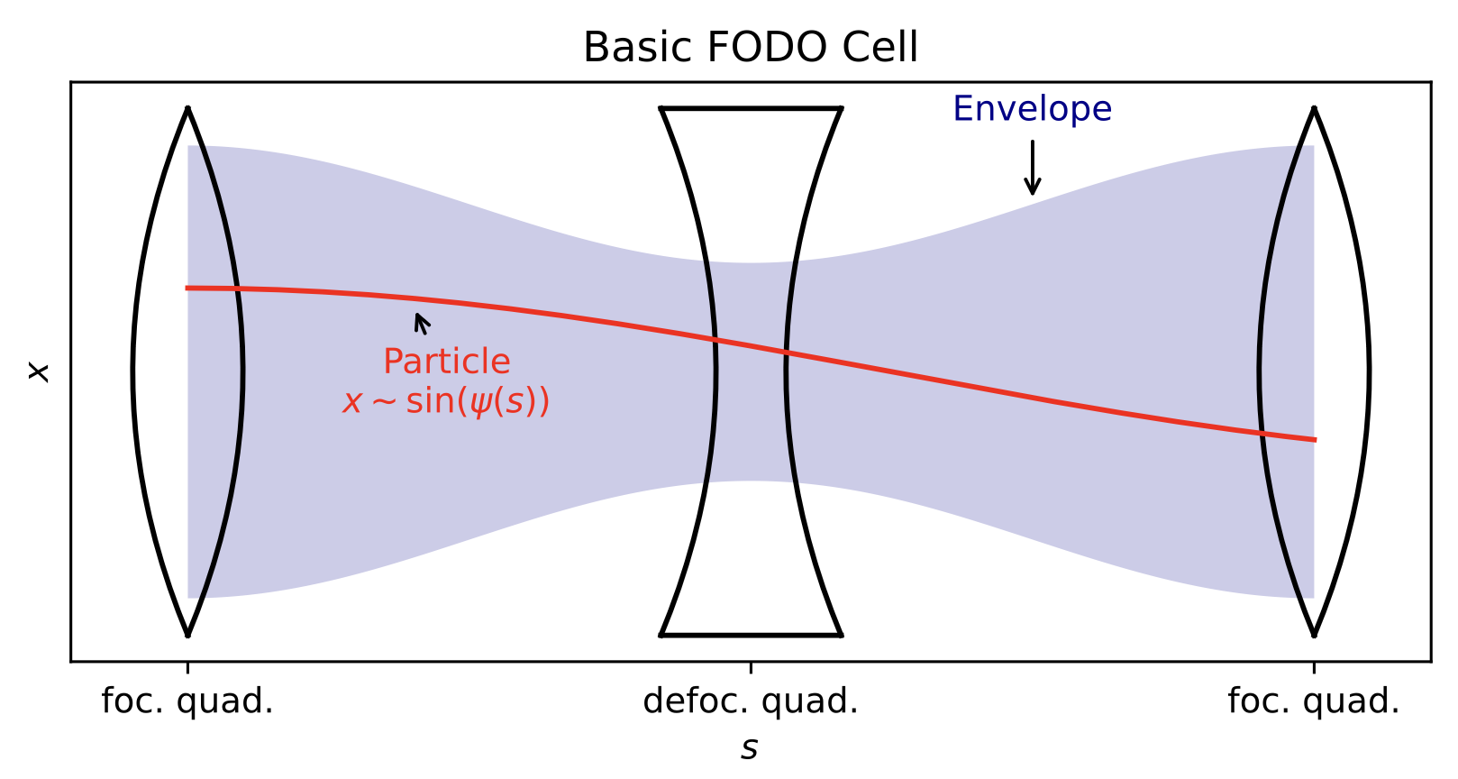
Local rms beam size $\sigma_{x,y}(s)$ determined by $\beta_{x,y}$-functions and particle distribution in action $J_{x,y}$:
$$\sigma_u(s)^2=\langle u(s)^2\rangle_\text{particles}=2\langle J_u\rangle\cdot\beta_u(s)$$
where $\langle \cdot \rangle_\text{particles}$ refers to averaging over the particle ensemble and $u=x,y$.
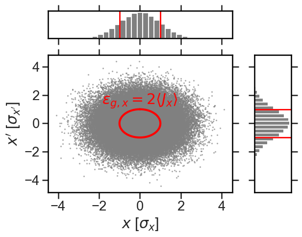
Defining the (geometric) rms emittance as $\epsilon_{g,u}=2\langle J_u\rangle$, one finds the rms beam size or beam envelope to vary with $s$ as
$$\sigma_u(s)=\sqrt{\epsilon_{g,u}\cdot\beta_u(s)}$$
The emittance $\epsilon_g$ is a measure for how spread out particles are in phase space. The rms ellipse spans an area of $\pi\epsilon_g$.
Stability of Solutions
Solutions of Hill equation pick up a factor $e^{\pm i \mu(L)}$ after one turn:
$$u(s+L)=\underbrace{\omega(s+L)}\limits_{\mathop{\equiv}\omega(s)}\cdot e^{\pm i\mu(s+L)} = \underbrace{\omega(s) \cdot e^{\pm i\mu(s)}}\limits_{\mathop{=}u(s)} \cdot e^{\pm i\mu(L)} = u(s)\cdot e^{\pm i \mu(L)}$$
In general, Floquet exponent $\mu(s)\in\mathbb{C}$ $\implies$ eigenvalues of one-turn matrix $\mathcal{M}_L$ are exactly:
$$\mathcal{M}_L \cdot \mathbf{u} = e^{\pm i \mu(L)} \cdot \mathbf{u}$$
$\implies$ For stable solutions $u$ (finite and bounded motion!), this must remain on the unit circle:
$$\left|e^{\pm i \mu(L)}\right| = 1 \quad \Longleftrightarrow \quad \mu(L)\in\mathbb{R}\quad \Longleftrightarrow \quad \mathbf{u}\rightarrow\text{oscillatory}$$
This corresponds to stable focusing in an accelerator with bounded oscillations around the equilibrium closed orbit.
In this case, $\mu(s)$ is a real and monotonically increasing function $\psi(s)$ along $s$, commonly referred to as phase advance.
Unstable Solutions
For a general complex-valued $\mu(L)=\psi + i\lambda$ with $\psi,\lambda\in\mathbb{R}$, one finds
$$u(s+L)=u(s)\cdot \underbrace{e^{\pm i \psi}}\limits_{\text{oscillatory!}} \cdot \underbrace{e^{\pm \lambda}}\limits_{\text{instability for }\lambda\mathop{\neq} 0}$$
This imaginary part of $\mu(s)$, $\lambda$, is the so-called Lyapunov exponent, often used as an observable / early indicator of dynamic chaos (see sextupole example in lecture 4)!
Because $\mathcal{M}_L$ is symplectic, per plane (2x2 matrix) we have $\det\mathcal{M}_L=1$ and hence eigenvalues $\lambda_1\cdot\lambda_2=1$. This means for the Lyapunov exponents: if one $\lambda<0$ appears, there must be another $\lambda>0$ leading to unstable motion.
The Betatron Tune
For stable motion, find the phase advance relation to the $\beta$-function:
$$\psi(s-s_0) = \int_{s_0}^s \frac{d\tilde{s}}{\beta(\tilde{s})}$$
In accelerator physics, refer to the phase advance per turn as the (betatron) tune $Q_{x,y}$:
$$\psi_x(L)=2\pi Q_x$$ $$\psi_y(L)=2\pi Q_y$$
The tune $Q_{x,y}$ counts the number of oscillations around the ring during one turn.
Further reading e.g. H. Wiedemann, "Particle Accelerator Physics" (p. 227ff)
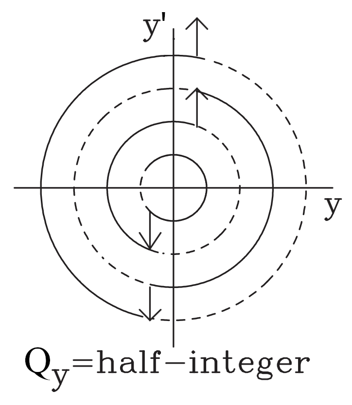
Resonances
For a stable accelerator setting, one finds that the phase advance should stay away from the resonance condition
$$\psi(n\cdot L)\neq 2\pi\cdot m\qquad \text{for } m,n\in\mathbb{N}$$
(i.e. after $n$ turns the phase advance becomes an integer multiple of $2\pi$), which is equivalent to demanding for the one-turn matrix
$$\begin{pmatrix}x\\ x'\end{pmatrix}_L = \mathcal{M}_{L,x} \begin{pmatrix}x\\ x'\end{pmatrix}_0 $$
to not become the unit matrix $\mathbb{1}$ after $n$ turns
$$\left(\mathcal{M}_{L,x}\right)^n \neq \begin{pmatrix} 1 & 0 \\ 0 & 1\end{pmatrix}$$
$\implies$ One needs to stay away from low-order resonances where this is fulfilled for low $n$, otherwise small disturbing kicks can add up coherently and lead to particle loss.
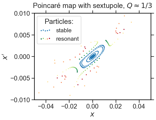
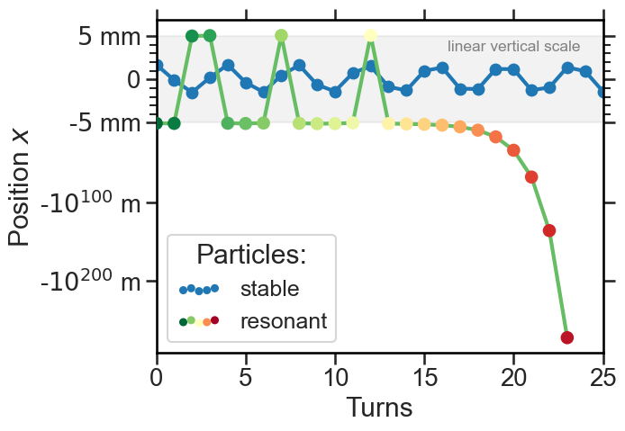
$\leadsto$ Try
Lecture 4 bonus exercise 6 with sextupole at k = 0.31 and mL = 1.8 settings to investigate the effect of a third-order resonance at $Q_x\approx 1/3$:
Part II: Optics and Twiss Parameters
Twiss Parameters
Particle motion along a magnetic lattice can be described by optical functions. A conventional parametrisation in accelerators uses the 3 local Twiss parameters $\beta_x, \alpha_x, \gamma_x$ (likewise for the vertical plane $y$). The Twiss parameters are linked via $\alpha_x(s)=-\cfrac{1}{2}\cfrac{d\beta_x(s)}{ds}$ and the identity $\beta_x\gamma_x = 1+\alpha_x^2$, i.e. there are only 2 degrees of freedom!
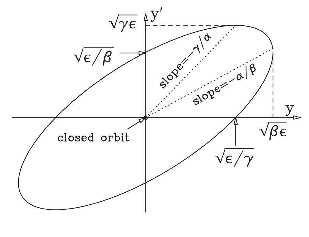
In phase space (on a Poincaré section), oscillating particles trace out an ellipse of area $\pi 2J$ which is described by the Twiss parameters (the image uses $\epsilon=2J$):
Periodic lattice
For a periodic lattice, the corresponding transfer matrix reads
$$\mathcal{M}_{\text{period,tw,}x} = \begin{pmatrix}\, \cos(\Phi_x) + \alpha_x\sin(\Phi_x) & \beta_x \sin(\Phi_x) \\ -\gamma_x \sin(\Phi_x) & \cos(\Phi_x) - \alpha_x\sin(\Phi_x) \end{pmatrix}$$
with the phase advance $\Phi_x$ over a full lattice period.
$\implies$ NB: the trace yields, as expected, $\mathrm{Tr}(\mathcal{M}_{\text{period,tw,}x})=2\cos(\Phi_x)$, as the $\alpha_x$ terms cancel.
Between any two locations $s_0$ and $s_1$, the solution of the Hill differential equation can be expressed in terms of the phase advance difference $\Delta \psi_x$ and the corresponding local Twiss parameters, $(\beta_x,\alpha_x,\gamma_x)$ at $s_0$ and $s_1$, respectively.
The Floquet transformation $F_0$ transforms the ellipse into a circle, where the rotation according to $\Delta\psi_x$ is applied, and then the inverse transformation $F_1^{-1}$ transforms back to real space according to the local optics at $s_1$:
$$\mathcal{M}_{\text{tw,}x}\bigr|_{s_1\leftarrow s_0} = \underbrace{\begin{pmatrix}\, \frac{1}{\sqrt{\beta_{x1}}} & 0 \\ \frac{\alpha_{x1}}{\sqrt{\beta_{x1}}} & \sqrt{\beta_{x1}} \end{pmatrix}^{-1}}\limits_{\mathop{\doteq} F_1{}^{-1}} \cdot \underbrace{\begin{pmatrix} \cos(\Delta \psi_x) & \sin(\Delta \psi_x) \\ -\sin(\Delta \psi_x) & \cos(\Delta \psi_x) \end{pmatrix}}\limits_{\mathop{\doteq} R} \cdot \underbrace{\begin{pmatrix} \frac{1}{\sqrt{\beta_{x0}}} & 0 \\ \frac{\alpha_{x0}}{\sqrt{\beta_{x0}}} & \sqrt{\beta_{x0}} \end{pmatrix}}\limits_{\mathop{\doteq}F_0}$$
Here, $F$ denotes the Floquet transformation matrix (from physical phase space $x-x'$ to normalised phase space $\eta-\eta'$) and $R\in\mathrm{SO}(2)$ a rotation matrix.
Exercise 1a: Compute Twiss Parameters
CERN's Methodical Accelerator Design code MAD-X (website) has been developed to simulate the optics in the Large Hadron Collider (LHC) with its two colliding beams. We will employ it to compute the optical Twiss functions for some magnetic lattices:
madx = Madx(stdout=sys.stdout)
  ++++++++++++++++++++++++++++++++++++++++++++
  +     MAD-X 5.09.03  (64 bit, Darwin)      +
  + Support: mad@cern.ch, http://cern.ch/mad +
  + Release   date: 2024.04.25               +
  + Execution date: 2026.05.06 21:58:19      +
  ++++++++++++++++++++++++++++++++++++++++++++
Define the following periodic beam line of $10\,$m length:
- focusing quadrupole centred at 3m (strength $k=0.1\,$m${}^{-2}$ and length $L=0.6\,$m)
- dipole sector bend centred at 5m (bending angle $\theta=\pi/8$ and length $L=0.6\,$m)
- defocusing quadrupole centred at 7m (strength $k=-0.5\,$m${}^{-2}$ and length $L=0.4\,$m)
madx.input('''
k1l_f := 0.1 * 0.6;  // inverse focal length qf
k1l_d := -0.5 * 0.4; // inverse focal length qd

qf: quadrupole, l = 0.6, k1 := k1l_f / 0.6;
qd: quadrupole, l = 0.4, k1 := k1l_d / 0.4;
dip: sbend, l = 0.6, angle := pi / 8;

seq1: sequence, l = 10;
qf, at = 3;
dip, at = 5;
qd, at = 7;
endsequence;
''')
True
madx.command.beam(particle='proton', energy=1) # energy is in GeV!
madx.use(sequence='seq1')

# output the Twiss parameters every 0.1m
madx.command.select(flag="interpolate", sequence="seq1", step=0.1)
True
Now we compute the periodic solution to the Hill equation (in terms of the Twiss parameters):
twiss = madx.twiss();
enter Twiss module

iteration:   1 error:   0.000000E+00 deltap:   0.000000E+00
orbit:   0.000000E+00  0.000000E+00  0.000000E+00  0.000000E+00  0.000000E+00  0.000000E+00

++++++ table: summ

            length             orbit5               alfa            gammatr
                10                 -0      0.09572878063        3.232054955

                q1                dq1            betxmax              dxmax
      0.2393933525      -0.4979445041        11.70243519        7.345182369

             dxrms             xcomax             xcorms                 q2
       6.588466214                  0                  0       0.2224798695

               dq2            betymax              dymax              dyrms
     -0.1070464578        11.39223223                  0                  0

            ycomax             ycorms             deltap            synch_1
                 0                  0                  0                  0

           synch_2            synch_3            synch_4            synch_5
                 0                  0                  0                  0

           synch_6            synch_8             nflips              dqmin
                 0                  0                  0                  0

       dqmin_phase
                 0
Let us investigate the optical functions along this periodic beam line (red areas mark quadrupoles, gray areas mark dipoles):
plot_twiss(twiss);

$\implies$ Periodic optics functions, values on the right at $s=10\,$m are equal to values on the left at $s=0\,$m!
$\leadsto$ Observe what happens to the $\beta_{x,y}$ functions at the locations of the quadrupoles (red areas)! Do you understand the direction into which the $\beta$-functions turn?
$\leadsto$ Observe what happens to the optics inside the dipole (gray area)! Do you understand why only the horizontal plane is affected and how it is affected?
Exercise 1b: Compare Tracking with Twiss and Betatron Matrices
We provide interpolation functions for any position $s$ given the MAD-X computed Twiss table $s-\beta_{x,y}-\alpha_{x,y}-\psi_{x,y}$:
beta_x = interp1d(twiss['s'], twiss['betx'], kind='linear')
alpha_x = interp1d(twiss['s'], twiss['alfx'], kind='linear')
psi_x = interp1d(twiss['s'], 2 * np.pi * twiss['mux'], kind='linear')
Define the Floquet transformation matrix and the rotation matrix for the Twiss transport matrix:
def F(beta, alpha):
    '''Floquet transformation matrix to normalised phase space.'''
    return np.array([
        [1 / np.sqrt(beta), 0],
        [alpha / np.sqrt(beta), np.sqrt(beta)]
    ])

def R(angle):
    '''Rotation matrix.'''
    return np.array([
        [np.cos(angle), np.sin(angle)],
        [-np.sin(angle), np.cos(angle)]
    ])

def M_tw(beta0, alpha0, beta1, alpha1, delta_psi):
    '''Transport matrix with Twiss parameters from index 0 to 1.'''
    F0 = F(beta0, alpha0)
    F1 = F(beta1, alpha1)
    F1inv = np.linalg.inv(F1)
    Rot = R(delta_psi)
    return F1inv.dot(Rot.dot(F0))
Prepare the tracking of a particle along this periodic beam line: once with betatron matrices for each element, once with the Twiss matrix!
# path length positions at edges of elements
s = [0, 3 - 0.6/2, 3 + 0.6/2, 5 - 0.6/2, 5 + 0.6/2, 7 - 0.4/2, 7 + 0.4/2, 10]
ds = np.diff(s)
# betatron matrices
d1 = M_drift(ds[0])
qf = M_quad_x(ds[1], 0.1)
d2 = M_drift(ds[2])
dip = M_dip_x(ds[3], 0.6 / (np.pi / 8)) # rho0 = L / angle
d3 = M_drift(ds[4])
qd = M_quad_x(ds[5], -0.5)
d4 = M_drift(ds[6])
# Twiss transport matrix
def M_tw_s0to1_x(s0, s1):
    '''Twiss matrix from s0 to s1 (evaluating Twiss parameters at these points!).'''
    return M_tw(
        beta_x(s0), alpha_x(s0),
        beta_x(s1), alpha_x(s1),
        psi_x(s1) - psi_x(s0)
    )
The initial horizontal coordinates of the particle at $s=0\,$m:
x_ini = 0.02
xp_ini = 0.01
Some plotting helper functions:
def scatter(s, x, label=None):
    plt.scatter([s], [x], c='red', s=30, marker='D', label=label)

def scatter_tw(s, x, label=None):
    plt.scatter([s], [x], c='cyan', s=40, marker='.', label=label)
Go for the tracking!
# track with betatron matrices from one element to the next:
scatter(0, x_ini, label='betatron matrix')

x, xp = track(d1, x_ini, xp_ini)
scatter(s[1], x)

x, xp = track(qf, x, xp)
scatter(s[2], x)

x, xp = track(d2, x, xp)
scatter(s[3], x)

x, xp = track(dip, x, xp)
scatter(s[4], x)

x, xp = track(d3, x, xp)
scatter(s[5], x)

x, xp = track(qd, x, xp)
scatter(s[6], x)

x, xp = track(d4, x, xp)
scatter(s[7], x)

# track with the Twiss transport matrix
scatter_tw(0, x_ini, label='Twiss matrix')
xt, xpt = x_ini, xp_ini
for i in range(len(s) - 1):
    M_tw_x = M_tw_s0to1_x(s[i], s[i + 1])
    xt, xpt = track(M_tw_x, xt, xpt)
    scatter_tw(s[i + 1], xt)

plt.xlabel('$s$ [m]')
plt.ylabel('$x$ [m]')
plt.legend(loc='lower right');

$\implies$ The transfer maps via the Twiss parameters $\beta_x(s), \alpha_x(s), \gamma_x(s)$ are identical to the element-by-element betatron matrices from the previous lecture! Both correctly describe the solution to the equation of motion (Hill differential equation!).
$\implies$ The advantage with $\mathcal{M}_\text{tw}$: only require one single matrix expression to describe solution at any location $s$! (Need to determine the optics functions / Twiss parameters first though!)
$\leadsto$ Are betatron matrices and the Twiss matrix also identical in the case of an unstable lattice?
Exercise 1c: Determine the Tune from Tracking and Compare to Computed Phase Advance
Let us track a particle with the compiled betatron matrix for a number of periods. We can determine the tune via Discrete Frequency Analysis (using NAFF) and then compare to the phase advance computed via the Twiss matrix approach:
M_period = qf.dot(d1)
M_period = d2.dot(M_period)
M_period = dip.dot(M_period)
M_period = d3.dot(M_period)
M_period = qd.dot(M_period)
M_period = d4.dot(M_period)
We need to record the oscillation for a useful number of turns:
nperiods = 128
rec_x = np.zeros(nperiods, dtype=float)
rec_x[0] = x_ini
Tracking:
x, xp = x_ini, xp_ini
for i in range(1, nperiods):
    x, xp = track(M_period, x, xp)
    rec_x[i] = x[0]
The horizontal motion at this location looks as follows:
plt.plot(rec_x)
plt.xlabel('Periods')
plt.ylabel('$x$ [m]');

We determine the tune via discrete frequency analysis, in this case using the PyNAFF library which implements the Numerical Analysis of Fundamental Frequencies algorithm:
tune = PyNAFF.naff(rec_x, turns=nperiods, nterms=1)[0, 1]
tune
np.float64(0.239334575934871)
$\implies$ This is the betatron tune of the particle (number of oscillations per period) measured via tracking data!
Now what about the phase advance from the full-period transfer matrix, $2\cos(\Phi_x)=\mathrm{Tr}(\mathcal{M})$ ?
trace = np.matrix.trace(M_period)

np.arccos(trace / 2)
np.float64(1.5041527952010787)
Convert from phase advance $\Phi_x$ to tune units $Q_x=\Phi_x/2\pi$:
np.arccos(trace / 2) / (2 * np.pi)
np.float64(0.23939335252174299)
Yes! $\implies$ The particle follows the same frequency in the tracking as determined via the Twiss matrix approach!
By the way, the phase advance or rather tune $Q=\psi\,/\,2\pi$ was also computed by MAD-X:
twiss.summary['q1']
0.2393933525
Exercise 2: Periodic Transport Matrices
Consider the following numerical (horizontal) transport matrices, each for a full period of a lattice.
Determine:
a) whether they are valid transport matrices (symplecticity)?
b) whether they represent stable betatron motion?
c) the covered phase advance $\Phi_x$ per lattice period (and the tune $Q_x=\Phi_x\,/\,2\pi$)?
How do the eigenvalues represent stability and phase advance? (check absolute values and complex phases, picture on the unit circle)
Hint: you might need the following functions for a given matrix M:
- determinant:
np.linalg.det(M) - trace:
np.trace(M) - eigenvalues:
np.linalg.eigvals(M) - arccos:
np.arccos(...) - sin:
np.sin(...) - absolute value:
np.abs(...) - phase $\phi$ (radiant units) from complex number $e^{i\phi}$:
np.angle(...) - matrix multiplication $M_1\cdot M_2$:
np.dot(M1, M2)orM1.dot(M2)
$$\mathcal{M}_1 = \begin{pmatrix} -0.03701215 & 0.19960535 \\ -5.04003498 & 0.16259319 \end{pmatrix}$$
M1 = np.array([
    [-0.03701215,  0.19960535],
    [-5.04003498,  0.16259319]
])
$$\mathcal{M}_2 = \begin{pmatrix} 0.5 & 13 \\ -0.0961538 & -0.5 \end{pmatrix}$$
M2 = np.array([
    [0.5,  13],
    [-0.09615385,  -0.5]
])
$\leadsto$ What happens to particles in this lattice after a short number of lattice periods? (Investigate by applying the transport matrix repetitively.)
$$\mathcal{M}_3 = \begin{pmatrix} 0.31803855 & 22.193583 \\ -0.1533821 & 0.93858321 \end{pmatrix}$$
M3 = np.array([
    [0.31803855,  22.193583],
    [-0.1533821,  0.93858321]
])
$$\mathcal{M}_4 = \begin{pmatrix} -0.75105652 & 0.69069571 \\ -0.02118063 & -1.31197933 \end{pmatrix}$$
M4 = np.array([
    [-0.75105652,  0.69069571],
    [-0.02118063, -1.31197933]
])
Part III: The FODO Cell
Exercise 3: Computing Optics of a FODO cell
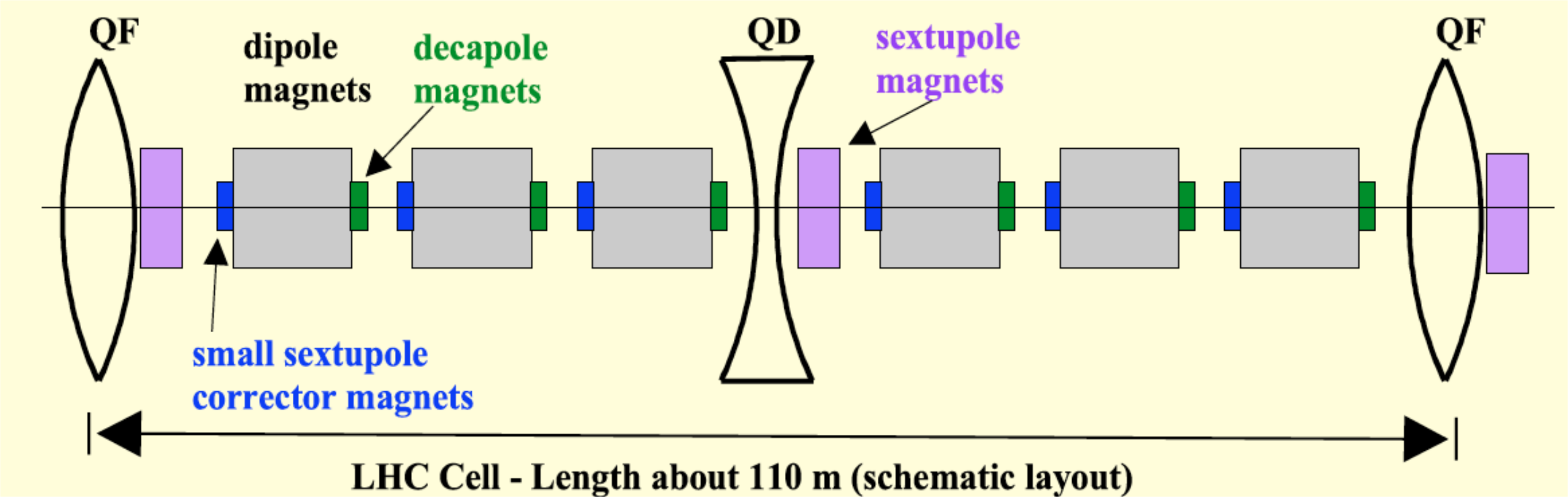
Consider a $110\,$m long FODO cell with $3.3\,$m long quadrupole magnets. A possible implementation might look like this (blue: dipoles, white: quadrupoles):
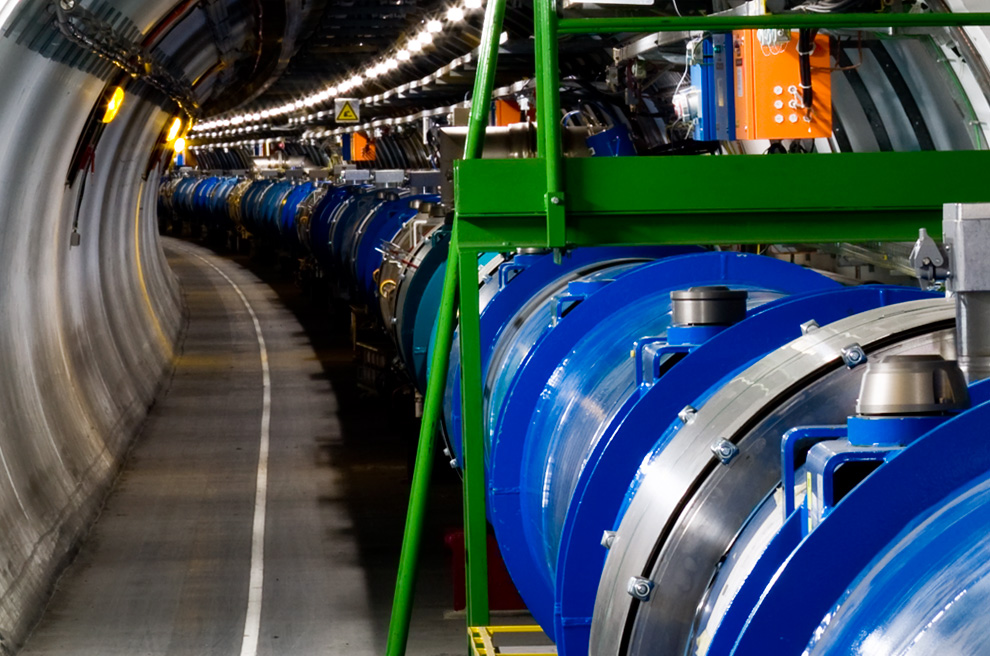
image by CERN
This time we start with a non-bending FODO cell, i.e. the dipoles switched off. (We will revisit this case with dipoles in lecture 6.)
Let us determine the optical functions, again via MAD-X:
madx = Madx(stdout=sys.stdout)
  ++++++++++++++++++++++++++++++++++++++++++++
  +     MAD-X 5.09.03  (64 bit, Darwin)      +
  + Support: mad@cern.ch, http://cern.ch/mad +
  + Release   date: 2024.04.25               +
  + Execution date: 2026.05.06 21:58:20      +
  ++++++++++++++++++++++++++++++++++++++++++++
We define the FODO cell with two quadrupoles of opposite strength, $k\cdot L=0.008\cdot 3.3\,$m${}^{-1}$, and with three dipoles in between each quadrupole. For the moment the dipoles are switched off (their bending angle $\theta=0$):
madx.input('''
k1l_f := 0.008 * 3.3;  // inverse focal length qf
k1l_d := -0.008 * 3.3; // inverse focal length qd
theta := 0;            // in LHC: 2 * pi / 1232;

qf2: quadrupole, l = 3.3 / 2, k1 := k1l_f / 3.3; // half a focusing quad
qd:  quadrupole, l = 3.3,     k1 := k1l_d / 3.3;
dip: sbend, l = 14.3, angle := theta;

fodo: sequence, l = 110;
qf2, at = 3.3 / 4;
dip, at = 12;
dip, at = 2 * 110 / 8;
dip, at = 110 / 2 - 12;
qd, at = 110 / 2;
dip, at = 110 / 2 + 12;
dip, at = 6 * 110 / 8;
dip, at = 110 - 12;
qf2, at = 110 - 3.3 / 4;
endsequence;
''')
True
madx.command.beam(particle='proton', energy=7e3) # energy is in GeV!
madx.use(sequence='fodo')

# output the Twiss parameters every 1m
madx.command.select(flag="interpolate", sequence="fodo", step=1)
True
We call the Twiss routine to compute the optics:
twiss = madx.twiss();
enter Twiss module

iteration:   1 error:   0.000000E+00 deltap:   0.000000E+00
orbit:   0.000000E+00  0.000000E+00  0.000000E+00  0.000000E+00  0.000000E+00  0.000000E+00

++++++ table: summ

            length             orbit5               alfa            gammatr
               110                 -0                  0                  0

                q1                dq1            betxmax              dxmax
      0.2518947018      -0.3220961047        186.9084848                  0

             dxrms             xcomax             xcorms                 q2
                 0                  0                  0       0.2518947018

               dq2            betymax              dymax              dyrms
     -0.3220961047        186.4581481                  0                  0

            ycomax             ycorms             deltap            synch_1
                 0                  0                  0                  0

           synch_2            synch_3            synch_4            synch_5
                 0                  0                  0                  0

           synch_6            synch_8             nflips              dqmin
                 0                  0                  0                  0

       dqmin_phase
                 0
The optics of the LHC FODO cell looks as follows:
plot_twiss(twiss, what='lhc')

$\leadsto$ Can you identify where the maximum and minimum of the transverse $\beta$-functions are located in the magnet lattice? What about the values of the $\alpha$-functions at these locations?
$\leadsto$ Can you explain the alternating-gradient focusing concept in terms of the $\beta$-functions?
Summary
- Hill Equation describes particle trajectories in periodic focusing (betatron motion)
- Phase advance and betatron tune
- Stable beam transport, lattice instability and resonances
- Optics / Twiss functions, $\beta$-function, rms emittance and rms beam size $\sigma=\sqrt{\beta\epsilon_g}$
- Periodic transport matrix, computing Twiss parameters and phase advance
- Betatron matrices and Twiss matrix provide 2 representations of identical solution to Hill differential equation
- Stability of periodic transport matrices
- Optics ($\beta$- and $\alpha$-functions) in a FODO cell