Integrating GPU libraries for fun and profit¶

...on extending and interfacing HPC simulation tools¶

Authors: Adrian Oeftiger and Martin Schwinzerl¶

PyHEP'20, see indico here $\nearrow$. See also rendered talk on github $\nearrow$ and source in github repo $\nearrow$.

Abstract¶

I have a high-performance number crunching tool with cool physics which simulates long-term on a GPU – how can I extend the inner loop by further cool physics, injected from the outside? In python this should be easy, right? But wait... we are sitting on device memory?

In this talk we explore how to tightly couple two libraries for high-performance computation of long-term beam dynamics, SixTrackLib and PyHEADTAIL. How can we design the interface between both libraries in terms of

(1) remaining on the python level,

(2) avoid losing performance due to device-to-host-to-device copies, and

(3) keeping both libraries as stand-alone packages?

The interface can be surprisingly simple, yet fully fledged... Let's go!

... the physics ...¶

Collective beam dynamics¶

3D particle motion $\leadsto$ 6 phase space coordinates: $$\mathbb{X}=(\underbrace{x, x'\vphantom{y'}}_{horizontal}, \underbrace{y, y'}_{vertical}, \underbrace{z, \delta\vphantom{y'}}_{longitudinal})$$

A beam $=$ state of $N$ macro-particles $=$ $6N$ values of phase space coordinates

Simulations:¶

typically up to $\mathcal{O}(10^6)$ macro-particles
accelerator elements to track through: up to $\mathcal{O}(1000)$
simulations can last up to $\mathcal{O}(10^6)$ turns
particle-to-particle interaction: binning, FFT, convolution, particle-in-cell, Poisson solvers

Requirements for simulation tools¶

long-term evolution $\leadsto$ double precision
heavy number crunching $\leadsto$ high-performance computing (HPC)
(in particular for collective effects i.e. particle-to-particle interaction)
iterative development, frequent update of accelerator models $\leadsto$ python

Single-particle vs. multi-particle dynamics¶

single-particle $\implies$ "tracking": particle motion due to external focusing (magnets and RF cavities)

multi-particle $\implies$ "collective effect kicks": direct and indirect particle-to-particle interaction

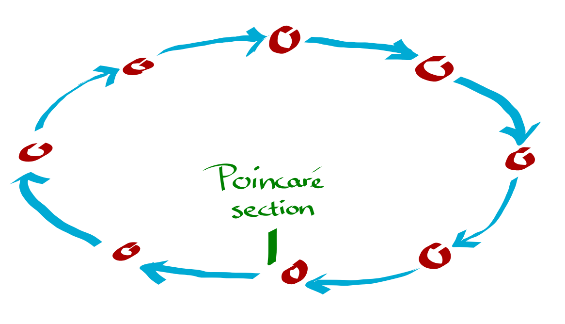Tracking around the accelerator ring

The `PyHEADTAIL` library¶

Python based code for simulating collective beam dynamics: github repo $\nearrow$

$\implies$ simplified matrix-based tracking

$\implies$ strong: detailed models for collective effect kicks

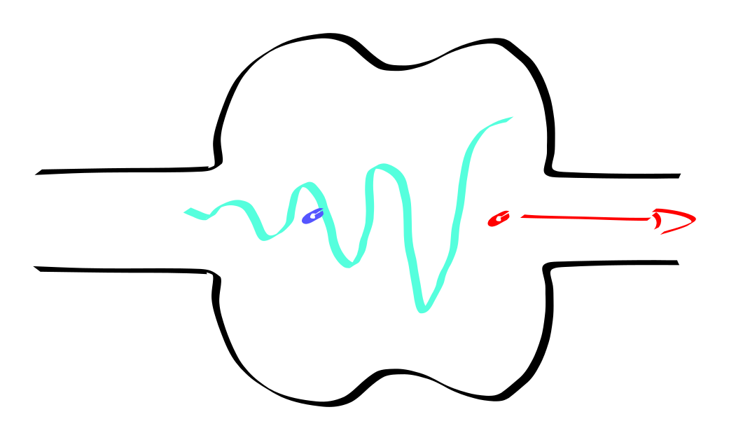Example for a kick: wakefield induced by leading particles imparting kicks on trailing particles

The `SixTrackLib` library¶

C templated code with Python API for simulating single-particle beam dynamics: github repo $\nearrow$

$\implies$ strong: advanced non-linear tracking

$\implies$ approximative / simplified models for collective effect kicks

Example for tracking: dipole magnets bend and quadrupole magnets (de-)focus particles

... the HPC part ...¶

`PyHEADTAIL` on the GPU¶

Concept presented on PyHEP'19 $\nearrow$, in short:

utilise duck typing to separate physics from back-end implementation
sandwich layer via context management and function redirection
(separate math dictionaries for CPU and GPU)
exploit GPU via PyCUDA (CuPy would work similarly)

# tracking loop in PyHEADTAIL:
with GPU(pyht_beam):
    for i in range(n_turns):
        for element in pyht_ring_elements:
            element.track(pyht_beam)

$\implies$ implement physics only once!
$\implies$ back-end details transparent to users / high-level developers

`SixTrackLib` on the GPU¶

Concept presented on PyHEP'19 $\nearrow$, in short:

Python API for dynamic interaction
C templating approach to separate physics from back-end implementation
- implementation in usual C for (single-core) CPU
- implementation in openCL for multi-core CPU and GPU (AMD, NVIDIA)
- implementation in CUDA for NVIDIA GPUs

# tracking kernel in SixTrackLib
trackjob = stl.TrackJob(stl_ring_elements, stl_beam, device='opencl:0.0')
trackjob.track_until(n_turns)

$\implies$ implement physics only once!
$\implies$ users launch "trackjobs" with just a single device keyword to switch architecture

... the quest ...¶

`SixTrackLib` $+$ `PyHEADTAIL` $=$ <3 ?¶

SixTrackLib $\rightarrow$ strong in advanced non-linear tracking

PyHEADTAIL $\rightarrow$ strong in collective effect kicks

$\implies$ SixTrackLib $+$ PyHEADTAIL $=$ strong in both?

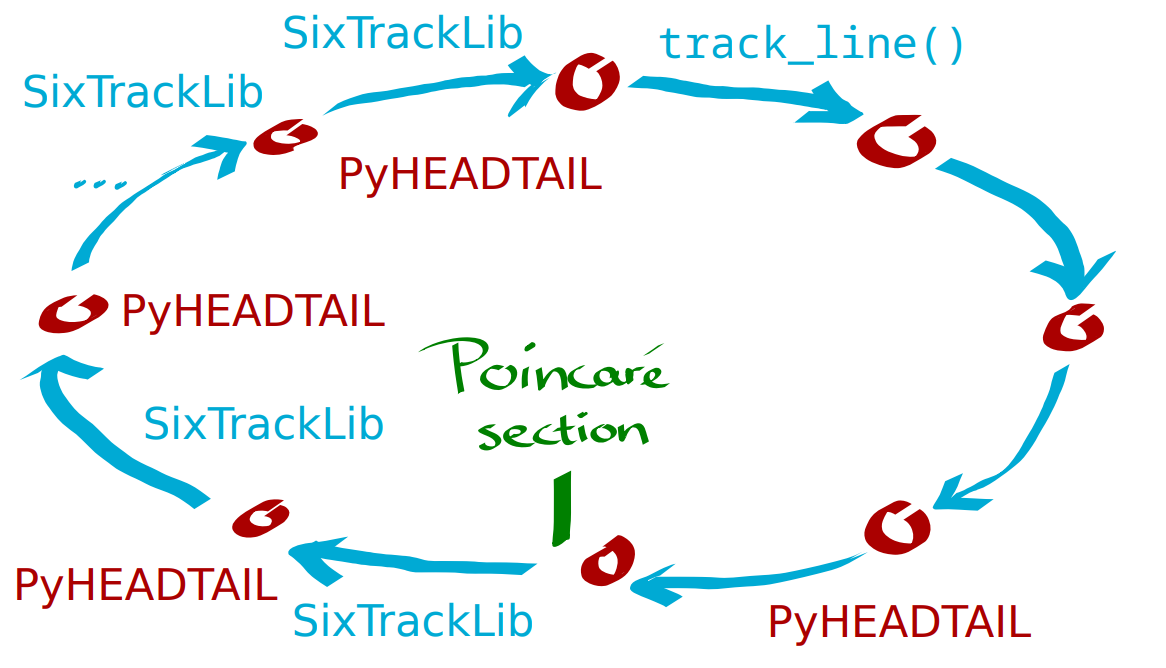Alternating SixTrackLib tracking and PyHEADTAIL kicking

... the questions ...¶

Situation:

PyHEADTAIL on the GPU lives in PyCUDA, managed from user script
SixTrackLib on the GPU manages its CUDA kernel invocation by itself
beam state data:
PyHEADTAIL uses PyCUDA.GPUArrays while SixTrackLib uses custom memory buffers

Critical aspects:

how to hand over the data between the two codes?
how to avoid GPU - CPU - GPU memory transfer?
can PyHEADTAIL's PyCUDA context interact with SixTrackLib's initialised context?
- visibility of memory to each other
- alternating kernel calls?
- flow control from python level?

... example simulation with `PyHEADTAIL` ...¶

... a coherent instability in the LHC ...¶

In [1]:

# import matplotlib, numpy, set pythonpath etc
from imports import *

from scipy.constants import m_p, c, e

Importing PyHEADTAIL:

In [2]:

# initialise CUDA context for PyHEADTAIL via pycuda
from pycuda import driver
context = driver.Device(0).make_context()

import PyHEADTAIL

PyHEADTAIL v1.14.1.21

In [3]:

#print current git commit for reference
import os
pyht_dir = os.path.dirname(PyHEADTAIL.__file__)
!printf "PyHEADTAIL " && cd $pyht_dir && git log | head -1

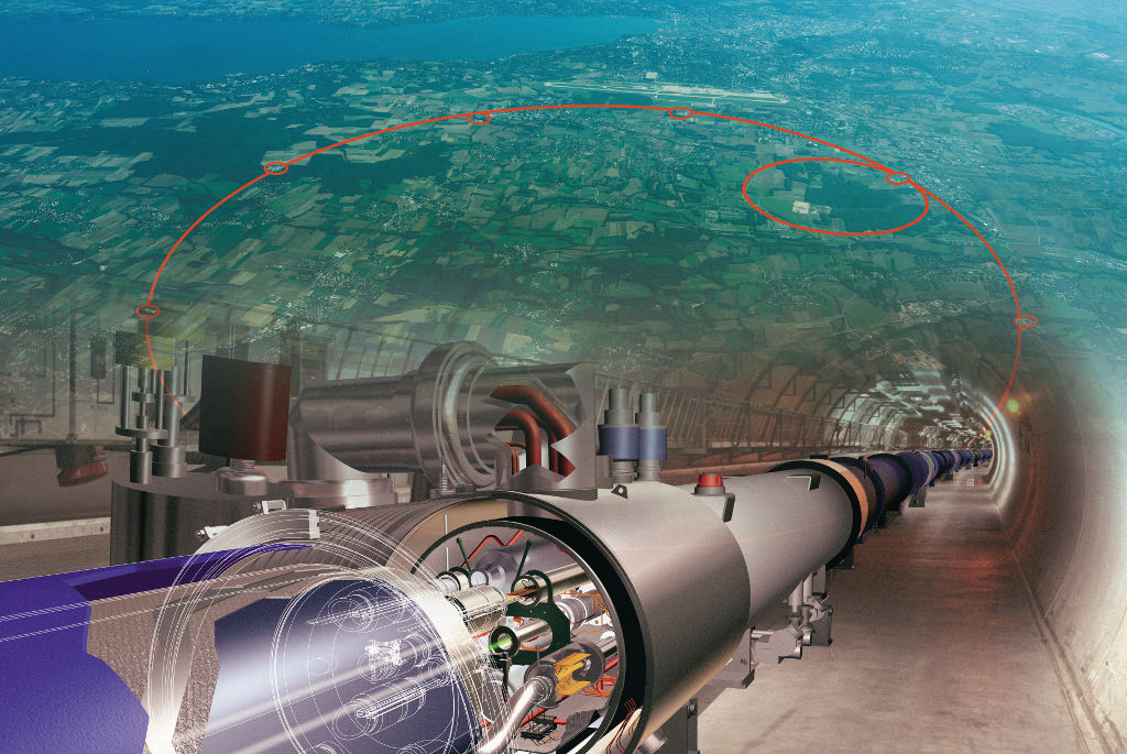
PyHEADTAIL commit 542cf33a3761f032a96d7dc1c84fd71e1e6e14e5

Setting up tracking around the LHC ring¶

Transverse tracking:

In [4]:

from PyHEADTAIL.trackers.transverse_tracking import TransverseMap
from PyHEADTAIL.trackers.detuners import Chromaticity

from pyheadtail_setup import transverse_map_kwargs, Q_x, Q_y

In [5]:

transverse_map = TransverseMap(
#     detuners=[Chromaticity(10, 10)],
    **transverse_map_kwargs,
)

Longitudinal tracking:

In [6]:

from PyHEADTAIL.trackers.longitudinal_tracking import RFSystems

from pyheadtail_setup import longitudinal_map_kwargs

In [7]:

longitudinal_map = RFSystems(**longitudinal_map_kwargs)

Setting up collective effect kick¶

Simulate wakefields in bunch via broad-band resonator:

In [8]:

from PyHEADTAIL.impedances.wakes import WakeField, CircularResonator
from PyHEADTAIL.particles.slicing import UniformBinSlicer

In [9]:

# responsible for binning the beam longitudinally:
slicer = UniformBinSlicer(n_slices=50, n_sigma_z=4)

# wakefield kick
resonator_wake = CircularResonator(
    R_shunt=100e6, frequency=0.8e9, Q=1,
)
wakefield = WakeField(slicer, resonator_wake)

Assembling the transport map around the LHC ring:¶

In [10]:

pyht_ring_elements = list(transverse_map) + [longitudinal_map, wakefield]

image reference: CMS-doc-5740-v1

Initialising the particle bunch¶

6D Gaussian distribution:

In [11]:

import pyht_streamless_slicing
from PyHEADTAIL.particles.generators import generate_Gaussian6DTwiss

from pyheadtail_setup import beam_kwargs

In [12]:

n_macroparticles = 10000
intensity = 1e11 * 5

np.random.seed(0)

pyht_beam = generate_Gaussian6DTwiss(
    macroparticlenumber=n_macroparticles,
    intensity=intensity,
    **beam_kwargs,
    **transverse_map.get_injection_optics(
        for_particle_generation=True),
)

A nicely Gaussian distributed bunch:

In [13]:

fig, ax = plt.subplots(1, 3, figsize=(12, 4))
plt.sca(ax[0])
plt.xlabel('$x$ [mm]')
plt.hist(pyht_beam.x * 1e3, bins=30);

plt.sca(ax[1])
plt.xlabel('$y$ [mm]')
plt.hist(pyht_beam.y * 1e3, bins=30);

plt.sca(ax[2])
plt.xlabel('$z$ [m]')
plt.hist(pyht_beam.z, bins=30);
plt.tight_layout()

Initial vertical bunch offset:

In [14]:

pyht_beam.y += 0.1 * pyht_beam.sigma_y()

Storing a blueprint of the initial bunch state for later:

In [15]:

slices0 = pyht_beam.get_slices(slicer, statistics=['mean_y'])

Let's go – simulating the LHC in `PyHEADTAIL` on the GPU:

In [16]:

from PyHEADTAIL.general.contextmanager import CPU, GPU
from PyHEADTAIL.general import pmath

In [17]:

n_turns = 500

# transfer to GPU
with GPU(pyht_beam):
    my = pmath.zeros(n_turns, dtype=float)
    
    # loop over turns
    for i in range(n_turns):
        # loop over elements around ring
        for element in pyht_ring_elements:
            element.track(pyht_beam)

        # record vertical bunch centroid amplitude
        my[i] = pyht_beam.mean_y()

In [18]:

my = pmath.ensure_CPU(my)

Outcome of our simulation?¶

In [19]:

plt.plot(my * 1e3)
plt.xlabel('Turns')
plt.ylabel(r'$\langle y \rangle$ [mm]')
plt.title('Vertical bunch centroid motion');

$\leadsto$ centre-of-mass of the bunch grows exponentially $\implies$ instability!

This transverse mode coupling instability develops along the bunch:

In [20]:

from imports import plot_intrabunch

plot_intrabunch(pyht_ring_elements, pyht_beam, slicer, slices0)

The LHC accelerator layout ("lattice") was simulated with a simple matrix tracking model in PyHEADTAIL.

In [21]:

pyht_beam = generate_Gaussian6DTwiss(
    macroparticlenumber=n_macroparticles,
    intensity=intensity,
    **beam_kwargs,
    **transverse_map.get_injection_optics(
        for_particle_generation=True),
)

In [22]:

pyht_ring_elements = list(transverse_map) + [longitudinal_map] # no wakefield

In [23]:

n_turns = 200

# transfer to GPU
with GPU(pyht_beam):
    sx = pmath.zeros(n_turns, dtype=float)
    
    # loop over turns
    for i in range(n_turns):
        # loop over elements around ring
        for element in pyht_ring_elements:
            element.track(pyht_beam)

        # record horizontal bunch size oscillation
        sx[i] = pyht_beam.sigma_x()

In [24]:

sx = pmath.ensure_CPU(sx)

In [25]:

plt.plot(sx * 1e3)
plt.xlabel('Turns')
plt.ylabel('$\sigma_x$ [mm]')
plt.title('Horizontal beam size oscillation');

... SixTrackLib can simulate the real lattice... shall we?

... example simulation with `SixTrackLib` ...¶

... tracking around the LHC ...¶

Importing SixTrackLib:

In [26]:

import sixtracklib as stl

In [27]:

# in absence of versioning, print current git commit for reference
stl_dir = os.path.dirname(stl.__file__)
!printf "SixTrackLib " && cd $stl_dir && git log | head -1

SixTrackLib commit 947643d56dd16b0106f9efd71510053bceef8c2d

Load the LHC lattice¶

In [28]:

stl_ring_elements = stl.Elements.fromfile(
    stl_dir + '/../../tests/testdata/lhc_no_bb/beam_elements.bin')

And add a monitor to record the motion of particles later when the tracking kernel is dispatched:

In [29]:

n_macroparticles = 1000
n_turns = 200

stl_ring_elements.BeamMonitor(
    start=0, num_stores=n_turns, max_particle_id=n_macroparticles - 1);

Initialise another `PyHEADTAIL` bunch...¶

In [30]:

np.random.seed(0)

pyht_beam = generate_Gaussian6DTwiss(
    macroparticlenumber=n_macroparticles,
    intensity=0,
    # the injection optics for this LHC lattice:
    alpha_x=2.2,
    beta_x=117,
    dispersion_x=-0.41,
    alpha_y=-2.7,
    beta_y=218,
    dispersion_y=-0.047,
    **beam_kwargs,
)

... and transfer the bunch to `SixTrackLib`¶

Initialise SixTrackLib particles object:

In [31]:

stl_beam = stl.Particles.from_ref(
    n_macroparticles, p0c=pyht_beam.p0 * c / e, 
    mass0=pyht_beam.mass * c**2 / e, q0=1)

And transfer PyHEADTAIL bunch coordinate arrays:

In [32]:

stl_beam.x[:] = pyht_beam.x
stl_beam.px[:] = pyht_beam.xp
stl_beam.y[:] = pyht_beam.y
stl_beam.py[:] = pyht_beam.yp
stl_beam.zeta[:] = pyht_beam.z
stl_beam.delta[:] = pyht_beam.dp

Actually, SixTrackLib particles hold a few more longitudinal coordinates just for convenience / rapid computation:

In [33]:

p0 = pyht_beam.p0
beta = pyht_beam.beta

restmass = pyht_beam.mass * c**2
restmass_sq = restmass**2
E0 = np.sqrt((p0 * c)**2 + restmass_sq)
p = p0 * (1 + pyht_beam.dp)
E = np.sqrt((p * c)**2 + restmass_sq)

gammai = E / restmass
betai = np.sqrt(1 - 1. / (gammai * gammai))

We also need to initialise them:

In [34]:

stl_beam.rpp[:] = 1. / (pyht_beam.dp + 1)
stl_beam.psigma[:] = (E - E0) / (beta * p0 * c)
stl_beam.rvv[:] = betai / beta

Tracking in `SixTrackLib`¶

With the accelerator lattice and the beam defined, go for trackjob:

In [35]:

trackjob = stl.TrackJob(stl_ring_elements, stl_beam, device='opencl:1.0')

In [36]:

trackjob.track_until(n_turns)
trackjob.collect();

$\implies$ the kernel to track all turns through all elements is dispatched to the GPU with the track_until call

Collecting the output¶

In [36]:

x = trackjob.output.particles[0].x
sigma_x = np.std(x.reshape(n_turns, n_macroparticles), axis=1)

In [37]:

plt.plot(1e3 * sigma_x, lw=1)
plt.xlabel('Turns')
plt.ylabel('$\sigma_x$ [mm]')
plt.title('Horizontal beam size oscillation');

$\implies$ SixTrackLib offers more complex kinetics than just a matrix ;-)

... well – let's try to unify, shan't we?

Integrating SixTrackLib tracking with wakefield kick from PyHEADTAIL

1 turn $=$ SixTrackLib tracks complete ring + 1 PyHEADTAIL wakefield kick

$\implies$ flow control on python level (which library takes over when)

idea:¶

for i in range(n_turns):
    # SixTrackLib:
    pyht_to_stl()
    trackjob.track_until(i)
    stl_to_pyht()
    # PyHEADTAIL
    wakefield.track(pyht_beam)

Memory transfer¶

So how to define pyht_to_stl() and stl_to_pyht()?

Let's start with

A) `SixTrackLib` to `PyHEADTAIL`.¶

$\implies$ take a GPU memory pointer and construct a PyCUDA.GPUArray

In [38]:

# fresh restart with PyCUDA
driver.Context.pop()
context = driver.Device(0).make_context()

In [39]:

import pycuda.gpuarray as gp

In [40]:

def provide_pycuda_array(gpu_ptr, length):
    return gp.GPUArray(length, dtype=np.float64, gpudata=gpu_ptr)

Approach¶

use SixTrackLib's CudaTrackJob for the dedicated CUDA implementation $\implies$ stay in CUDA in both codes (no openCL)
prepare some GPU memory as an example in SixTrackLib
build a PyCUDA array around this memory for PyHEADTAIL

In [41]:

stl_beam = stl.Particles.from_ref(n_macroparticles)

In [42]:

type(stl_beam.x)

Out[42]:

numpy.ndarray

In [43]:

stl_beam.x[:] = np.arange(0, 1, 1./n_macroparticles)

In [44]:

stl_beam.x[:10]

Out[44]:

array([0.   , 0.001, 0.002, 0.003, 0.004, 0.005, 0.006, 0.007, 0.008,
       0.009])

In [45]:

stl_ring_elements = stl.Elements.fromfile(
    stl_dir + '/../../tests/testdata/lhc_no_bb/beam_elements.bin')

# allocates GPU memory and fills it i.a. with the stl_beam.x array
cuda_trackjob = stl.CudaTrackJob(stl_ring_elements, stl_beam)

Retrieve location of stl_beam.x within particles buffer on GPU, i.e. memory pointer:

In [46]:

cuda_trackjob.fetch_particle_addresses()
ptrs = cuda_trackjob.get_particle_addresses()

In [47]:

ptrs.contents.x

Out[47]:

140315499479216

In [48]:

x_gpu = provide_pycuda_array(ptrs.contents.x, n_macroparticles)

In [49]:

x_gpu[:10]

Out[49]:

array([0.   , 0.001, 0.002, 0.003, 0.004, 0.005, 0.006, 0.007, 0.008,
       0.009])

In [50]:

type(x_gpu)

Out[50]:

pycuda.gpuarray.GPUArray

$\implies$ cool, we can construct a PyCUDA array from GPU memory – allocated and filled through SixTrackLib!

$\implies$ direction SixTrackLib to PyHEADTAIL is covered!

B) `PyHEADTAIL` to `SixTrackLib`¶

The GPUArrays constructed during a PyHEADTAIL track call need not be the same memory location as before:

In [51]:

# simulate some tracking update:
x_pyht_tracked = x_gpu**2 + 1
x_pyht_tracked[:10]

Out[51]:

array([1.      , 1.000001, 1.000004, 1.000009, 1.000016, 1.000025,
       1.000036, 1.000049, 1.000064, 1.000081])

In [52]:

assert int(x_pyht_tracked.gpudata) != int(x_gpu.gpudata)
int(x_pyht_tracked.gpudata), int(x_gpu.gpudata)

Out[52]:

(140315499776000, 140315499479216)

$\implies$ copy the data back into the fixed buffer in SixTrackLib!

In [53]:

driver.memcpy_dtod(
    dest=ptrs.contents.x, 
    src=x_pyht_tracked.gpudata,
    size=x_pyht_tracked.nbytes
)

Let's check the buffer in SixTrackLib for the update:

In [54]:

provide_pycuda_array(ptrs.contents.x, n_macroparticles)[:10]

Out[54]:

array([1.      , 1.000001, 1.000004, 1.000009, 1.000016, 1.000025,
       1.000036, 1.000049, 1.000064, 1.000081])

Transfer data within SixTrackLib back to CPU:

In [55]:

cuda_trackjob.collect_particles()

Out[55]:

<sixtracklib.cuda.CudaTrackJob at 0x7f9f944f6ac8>

In [56]:

stl_beam.x[:10], type(stl_beam.x)

Out[56]:

(array([1.      , 1.000001, 1.000004, 1.000009, 1.000016, 1.000025,
        1.000036, 1.000049, 1.000064, 1.000081]), numpy.ndarray)

$\implies$ indeed, the buffer has been filled with the updated values of x!

And we can collect the updated data back to the CPU memory from the GPU device!

Finally – let's plug everything together!

Please: restart the notebook kernel to avoid any CUDA context mess (vs. openCL etc).

In [1]:

from imports import *

from pycuda.autoinit import context
from pycuda import driver
import pycuda.gpuarray as gp

from PyHEADTAIL.general.contextmanager import GPU
from PyHEADTAIL.general import pmath
from PyHEADTAIL.impedances.wakes import WakeField, CircularResonator
from PyHEADTAIL.particles.slicing import UniformBinSlicer
import pyht_streamless_slicing
from PyHEADTAIL.particles.generators import generate_Gaussian6DTwiss

import sixtracklib as stl

import os
stl_dir = os.path.dirname(stl.__file__)

from pyheadtail_setup import beam_kwargs
from scipy.constants import m_p, c, e

def provide_pycuda_array(gpu_ptr, length):
    return gp.GPUArray(length, dtype=np.float64, gpudata=gpu_ptr)

PyHEADTAIL v1.14.1.21

The beam (containers):¶

In [2]:

n_macroparticles = 10000
intensity = 1e11 * 50

np.random.seed(0)

pyht_beam = generate_Gaussian6DTwiss(
    macroparticlenumber=n_macroparticles,
    intensity=intensity,
    # the injection optics for this LHC lattice:
    alpha_x=2.2,
    beta_x=117,
    dispersion_x=-0.41,
    alpha_y=-2.7,
    beta_y=218,
    dispersion_y=-0.047,
    **beam_kwargs,
)

In [3]:

stl_beam = stl.Particles.from_ref(
    n_macroparticles, p0c=pyht_beam.p0 * c / e, 
    mass0=pyht_beam.mass * c**2 / e, q0=1)

The accelerator:¶

In [4]:

# SixTrackLib tracking part:
stl_ring_elements = stl.Elements.fromfile(
    stl_dir + '/../../tests/testdata/lhc_no_bb/beam_elements.bin')

cuda_trackjob = stl.CudaTrackJob(stl_ring_elements, stl_beam)

In [5]:

# PyHEADTAIL wakefield kick part:
slicer = UniformBinSlicer(n_slices=50, n_sigma_z=4)
resonator_wake = CircularResonator(R_shunt=100e6, frequency=0.8e9, Q=1)
wakefield = WakeField(slicer, resonator_wake)

Preparation for the GPU device data transfers:¶

Storing the SixTrackLib buffer pointers:

In [6]:

cuda_trackjob.fetch_particle_addresses()
ptrs = cuda_trackjob.get_particle_addresses()

pointers = {
    'x': provide_pycuda_array(ptrs.contents.x, n_macroparticles),
    'px': provide_pycuda_array(ptrs.contents.px, n_macroparticles),
    'y': provide_pycuda_array(ptrs.contents.y, n_macroparticles),
    'py': provide_pycuda_array(ptrs.contents.py, n_macroparticles),
    'z': provide_pycuda_array(ptrs.contents.zeta, n_macroparticles),
    'delta': provide_pycuda_array(ptrs.contents.delta, n_macroparticles),
    'rpp': provide_pycuda_array(ptrs.contents.rpp, n_macroparticles),
    'psigma': provide_pycuda_array(ptrs.contents.psigma, n_macroparticles),
    'rvv': provide_pycuda_array(ptrs.contents.rvv, n_macroparticles),
}

In [7]:

def memcpy(dest, src):
    '''Device memory copy from GPUArray src to GPUArray dest.'''
    driver.memcpy_dtod_async(dest.gpudata, src.gpudata, src.nbytes)

Function for PyHEADTAIL to SixTrackLib memory transfer:

In [8]:

from pycuda import cumath

def pyht_to_stl(pyht_beam):
    memcpy(pointers['x'], pyht_beam.x)
    memcpy(pointers['px'], pyht_beam.xp)
    memcpy(pointers['y'], pyht_beam.y)
    memcpy(pointers['py'], pyht_beam.yp)
    memcpy(pointers['z'], pyht_beam.z)
    memcpy(pointers['delta'], pyht_beam.dp)

    # further longitudinal coordinates of SixTrackLib
    rpp = 1. / (pyht_beam.dp + 1)

    restmass = pyht_beam.mass * c**2
    restmass_sq = restmass**2
    E0 = np.sqrt((pyht_beam.p0 * c)**2 + restmass_sq)
    p = pyht_beam.p0 * (1 + pyht_beam.dp)
    E = cumath.sqrt((p * c) * (p * c) + restmass_sq)
    psigma =  (E - E0) / (pyht_beam.beta * pyht_beam.p0 * c)

    gamma = E / restmass
    beta = cumath.sqrt(1 - 1. / (gamma * gamma))
    rvv = beta / pyht_beam.beta

    memcpy(pointers['rpp'], rpp)
    memcpy(pointers['psigma'], psigma)
    memcpy(pointers['rvv'], rvv)
    
    # PyCUDA context:
    context.synchronize()

Function for SixTrackLib to PyHEADTAIL memory transfer:

In [9]:

def stl_to_pyht(pyht_beam):
    # barrier to make sure any previous
    # SixTrackLib kernels have finished 
    cuda_trackjob.collectParticlesAddresses()
    
    pyht_beam.x = pointers['x']
    pyht_beam.xp = pointers['px']
    pyht_beam.y = pointers['y']
    pyht_beam.yp = pointers['py']
    pyht_beam.z = pointers['z']
    pyht_beam.dp = pointers['delta']

Ready for tracking:¶

In [10]:

n_turns = 11

with GPU(pyht_beam):
    my = pmath.zeros(n_turns, dtype=float)
    
    for i in range(n_turns):
        # SixTrackLib:
        pyht_to_stl(pyht_beam)
        cuda_trackjob.track_until(i)
        stl_to_pyht(pyht_beam)
        # PyHEADTAIL
        wakefield.track(pyht_beam)
        
        # record vertical bunch centroid amplitude
        my[i] = pyht_beam.mean_y()

In [11]:

my = pmath.ensure_CPU(my)

Simulation Results¶

$\implies$ strong instability, this time with realistic lattice:

In [12]:

plt.plot(my * 1e3)
plt.xlabel('Turns')
plt.ylabel(r'$\langle y \rangle$ [mm]')
plt.title('Vertical bunch centroid motion');

Along with the same type of displacement pattern along the bunch:

In [13]:

slices = pyht_beam.get_slices(slicer, statistics=True)
plt.plot(slices.z_centers, slices.mean_y * slices.n_macroparticles_per_slice)
plt.xlabel('$z$ [m]')
plt.ylabel('BPM signal')
plt.title('Vertical intra-bunch motion');

... Conclusions!¶

You have seen in action

a duck-typing approach to GPU computing with PyCUDA: the PyHEADTAIL library
a templated library supporting openCL and CUDA for GPU computing: the SixTrackLib library
a reunion of both:
- remaining on GPU device memory (avoid CPU transfer)
- alternating kernel calls from both libraries to update the bunch state
- flow control from python level

Advantages:

rapid adjustment of physics model possible
- python level avoids person-hours in development
both libraries remain stand-alone simulation tools
- avoid tight integration
profit from GPU speed-up as long as simulated physics is "heavy"
- heavy track functions $\implies$ marginal python overhead
CUDA offers unified memory $\implies$ extend to several GPU devices!

Disadvantages:

interface needs low-level pointer arithmetic on the GPU
need to be careful with memory deallocation ("which context does the allocated memory belong to")

Outlook¶

This notebook: just a mere example, not the usual use-case but fast enough for a demo

$\implies$ "starters" menu of ...

"1 turn $=$ SixTrackLib tracks complete ring + 1 PyHEADTAIL wakefield kick"

... can be generalised to have arbitrarily many stops during the ring tracking – at the expense of a new SixTrackLib tracking API: trackjob.track_line(i_from, i_to)

Here you find a more complex / realistic simulation example $\nearrow$.

Many thanks, we hope you enjoyed!¶