S35 Particle Detectors and Accelerators
Accelerator Physics by Professor Adrian Oeftiger
Lecture 2: Acceleration and Bunching
Run this notebook online!
Interact and run this jupyter notebook online:
Also find this lecture rendered as HTML slides on github $\nearrow$ along with the source repository $\nearrow$.
Run this first!
Imports and modules:
from config import np, plt, plot_rfwave
%matplotlib inline
Refresher!
- Intro to Accelerators
- similarities to plasma physics, importance of external fields
- rf cavities, dipole and quadrupole magnets
- Accelerator Types
- linacs, cyclotrons, synchrotrons, plasma accelerators
- Facilities & Applications
- light sources: Diamond
- neutron spallation sources: ISIS
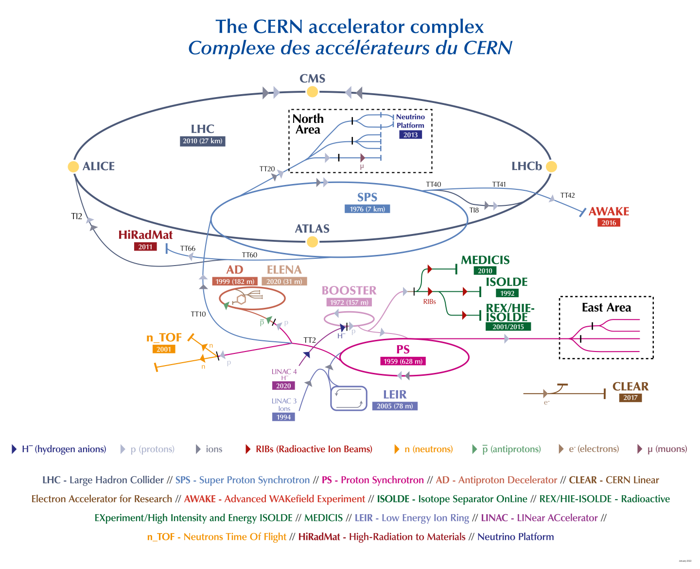
- high-energy physics: CERN
- Time Scales
Today!
- Basics: Relativistic particles in EM fields
- RF (Radio-Frequency) Cavities
- Longitudinal Beam Dynamics (Tracking Equations) in a Linac:
- Energy Gain
- Longitudinal Drift
A Relativistic Particle
Relativistic particle of rest mass $m_0$ at velocity $\mathbf{v}$ features momentum
$$p=|\mathbf{p}|=|\gamma m_0 \mathbf{v}| = \gamma m_0 \beta c$$
where
$$\begin{cases} c&\text{: speed of light in vacuum,}\qquad &c&\doteq 2.998\times 10^8 \text{m/s} \\[0.3em] \beta&\text{: particle speed in units of }c,\qquad&\beta&\doteq |\mathbf{v}/c| < 1 \\ \gamma&\text{: relativistic Lorentz factor,}\qquad &\gamma&\doteq\cfrac{1}{\sqrt{1 - \beta^2}} > 1 \end{cases}$$
Total energy defined by: $\qquad E_{\text{tot}}=\gamma m_0 c^2$
and related to momentum $p$ by the relativistic equation: $\qquad E_{\text{tot}}^2=\bigl(m_0c^2\bigr)^2 + (pc)^2$
Lorentz Force
Utilise electromagnetic fields $(\mathbf{E},\mathbf{B})$ to exert Lorentz force $\mathbf{F}_L$ on particle of charge $q$:
$$\frac{d\mathbf{p}}{dt} = \mathbf{F} = q\,(\mathbf{E}+\mathbf{v}\times\mathbf{B})$$
Deriving relativistic equation by time $t$ and using definition of $E_\text{tot}$:
$$\implies E_\text{tot} \frac{dE_\text{tot}}{dt} = c^2\cdot\mathbf{p}\cdot \frac{d\mathbf{p}}{dt} = c^2\cdot \mathbf{p}\cdot\mathbf{F}_L$$
$$\stackrel{/E_\text{tot}}{\implies} \frac{dE_\text{tot}}{dt} = \mathbf{v}\cdot\mathbf{F}_L = q\cdot \mathbf{v}\cdot(\mathbf{E}+\underbrace{\mathbf{v}\times \mathbf{B}}\limits_\text{cancels}) = q\cdot \mathbf{v}\cdot\mathbf{E}$$
Frenet-Serret Coordinate System
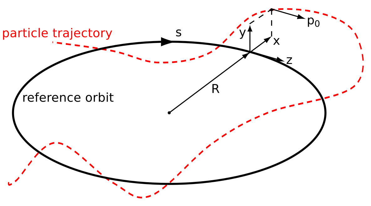
Particle moves along reference path parametrised by length $s$ with velocity
$$\mathbf{v}_s = \frac{d\mathbf{s}}{dt}$$
Phase space coordinates with respect to reference particle at $|\mathbf{p}|=p_0$ moving with time $t$:
| Plane | Coordinate (Offset) | Momentum |
|---|---|---|
| Horizontal | $x$ | $x'\doteq\frac{dx}{ds}$ |
| Vertical | $y$ | $y'\doteq\frac{dy}{ds}$ |
| Longitudinal | $z$ | $\delta\doteq\frac{p_z-p_0}{p_0}$ long. momentum deviation |
How to Accelerate?
Let us look at how the particle energy may change along $s$.
$$\implies \frac{dE_{\mathrm{tot}}}{ds} = \frac{1}{v_s} \frac{dE_{\mathrm{tot}}}{dt} = q \cdot \frac{\mathbf{v}}{v_s}\cdot \mathbf{E} = q \cdot \Bigl(\underbrace{\frac{v_z}{v_s}}\limits_{\color{red}{\mathop{\approx}1}}E_z + \underbrace{\frac{v_x}{v_s}}\limits_{\color{red}{\mathop{\approx}\frac{dx}{ds}\mathop{\equiv}x'}}\cdot E_x + \underbrace{\frac{v_y}{v_s}}\limits_{\color{red}{\mathop{\approx}\frac{dy}{ds}\mathop{\equiv}y'}}\cdot E_y \Bigr)$$
Here "$\approx$" is referred to as $\rightarrow$ "paraxial approximation".
Accelerate!
3 (+1) typical ways to supply $E_z$:
DC field, single passage!
$\rightarrow$ electrostatic accelerators: few MV/m before breakdownAC field: travelling wave rf cavities
$\rightarrow$ ultra-relativistic particles (typically electrons)AC field: resonator / standing wave rf cavities:
$\rightarrow$ most versatile standard (International Linear Collider project: 35 MV/m)
(+4. plasma wakefields, single passage!)
$\rightarrow$ ultra-relativistic particles (typically electrons), 100'000 MV/m
Part I: Momentum / Energy Gain
Longitudinal phase space: $(z, {\color{red}{\delta}})$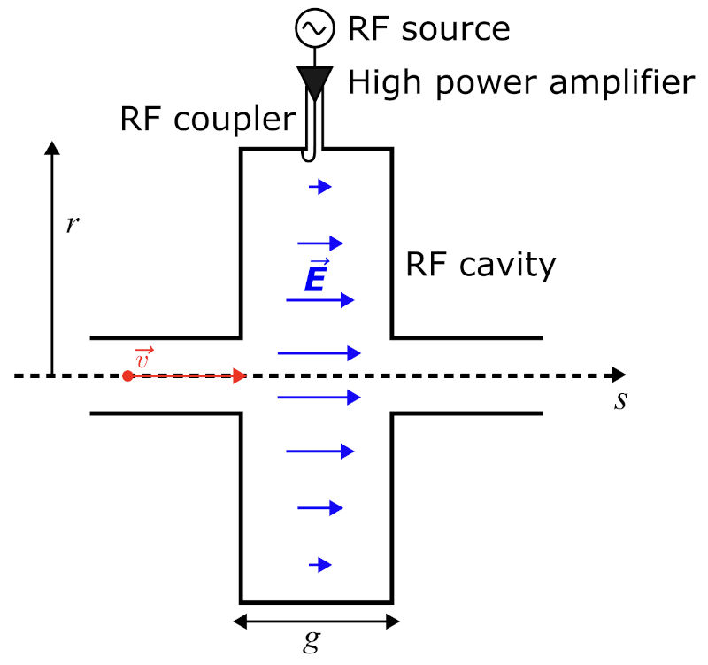
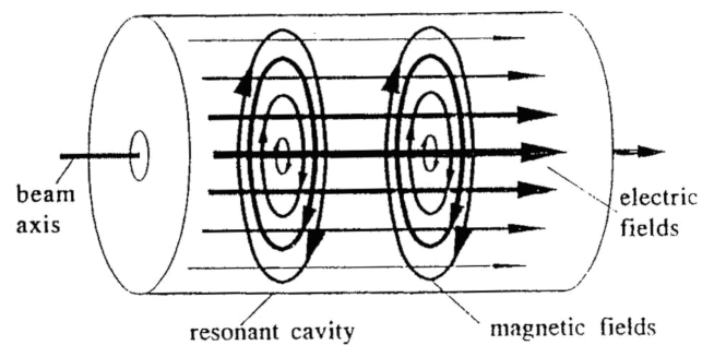
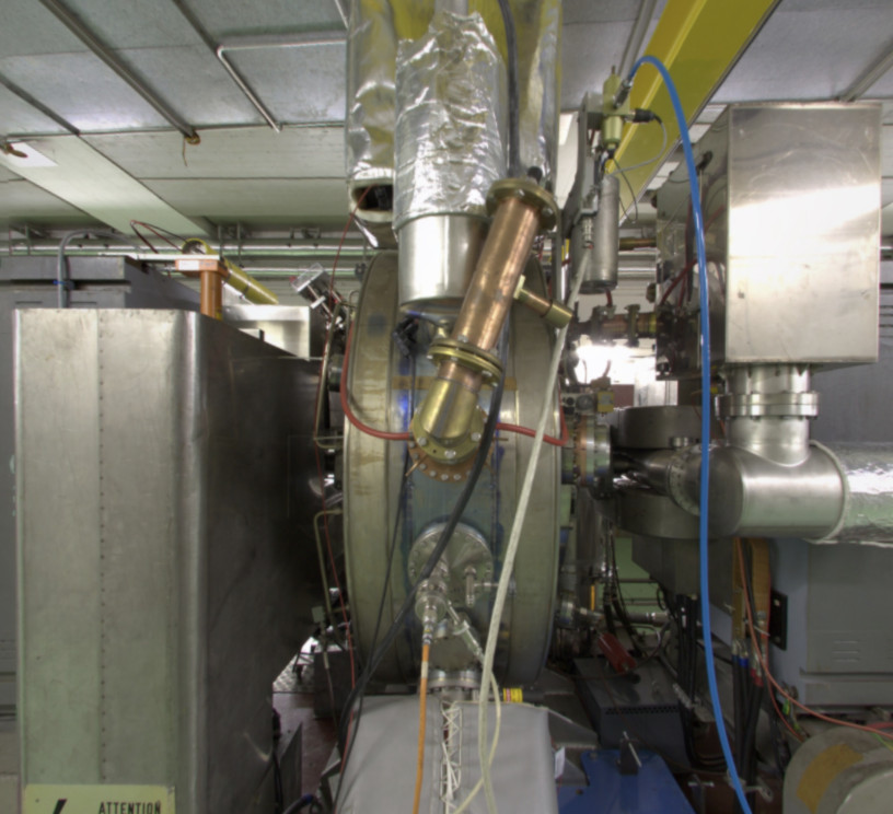
Standing-wave RF Cavities
Confine electromagnetic wave in a resonating cavity to provide oscillatory $E_z$ along axis:
$$\mathbf{E}(\mathbf{r},s,t)=E_{z,0}(\mathbf{r},s)\,\sin(\omega_\text{rf}\,t)\,\mathbf{e}_z$$
A low-power RF signal is amplified and coupled to the cavity to maintain and control amplitude of the RF wave with respect to the beam.
Exact field distribution $E_{z,0}(\mathbf{r},s)$ and RF (angular) frequency $\omega_\text{rf}=2\pi f_\text{rf}$ depend on cavity geometry. Typically TM${}_{010}$ is used as main accelerating mode for optimal $E_z$ along axis ($\Rightarrow$ magnetic field vanishes on-axis).
images by A. Lasheen and S. Tavernier
RF Voltage
Consider a particle of charge $q$ travelling along cavity axis $s$ while time $t$ passes:
$$E_z(s, t) = E_{z,0}(s) \cdot \sin\bigl(\omega_{\text{rf}}\, t + \varphi_s\bigr)$$
Here, $\varphi_s$ refers to synchronous phase at arrival of "synchronous" reference particle. The RF wave voltage amplitude is given by:
$$V_0 = \int\limits_{-\infty}^{+\infty} ds\,\left|E_{z,0}(s)\right|$$
(Hypothetical) maximum energy gain of particle during passage would be $\Delta W = |q|\cdot V_0$.
Transit-time Factor
Real energy gain for a particle $\Delta W$ reduces due to inevitable field variation during gap transit.
$\implies$ Transit-time factor:
$$ T = \frac{\text{energy gain of particle with }v=\beta c}{\text{maximum energy gain (particle with }v\rightarrow\infty\text{)}} \leq 1 $$
Effective RF voltage seen by particles is $V=V_0T$.
Energy Gain by RF Cavity
Reference beam energy increases as determined by synchronous phase $\varphi_s$,
$$\Delta W_0 = q V\cdot\sin(\varphi_s)$$
Real particles travel at a longitudinal distance $z = s - \beta c t$ to synchronous particle. They experience a "kick" at phase $\varphi = \omega_{\text{rf}}\,t = \varphi_s - \cfrac{\omega_{\text{rf}} z}{\beta c}$ with an energy gain of $\Delta W = q V\cdot \sin(\varphi)$.
Expressed as an energy distance $\Delta E$ to the synchronous particle, $\Delta E=E_{\text{tot}} - E_{\text{tot},0}$, the discrete energy update of an arbitrary particle passing through an RF cavity becomes
$$\begin{align} \Delta E|_{\text{after}} &= \Delta E|_{\text{before}} + \Delta W - \Delta W_0 \\ &= \Delta E|_{\text{before}} + q V\cdot \bigl(\sin(\varphi) - \sin(\varphi_s)\bigr) \end{align}$$
Phase or Longitudinal Focusing
Phase focusing principle (classical regime, see later), resulting in bunched beam:
- particle with $\varphi>\varphi_s$ arrives later and has $\color{blue}{\delta < 0}$:
needs to be accelerated towards synchronous particle! - particle with $\varphi<\varphi_s$ arrives early and has $\color{orange}{\delta > 0}$:
needs to be decelerated towards synchronous particle!
plot_rfwave(phi_s=0.5); # change phi_s and explore

Comprehension Questions
- Consider an ensemble of particles distributed in $\varphi$ around the (hypothetical) synchronous particle at $\varphi_s=30\,\text{deg}$. Assume linear drifts (constant momentum) in between many rf cavities along $s$. What qualitative type of motion of the ensemble would you expect in phase space along an extended distance?
- What would happen to a slower and faster particle, respectively, if $\varphi_s$ was moved to $\pi-\varphi_s$? How would the motion of the particle ensemble change accordingly?
Linear Accelerators / Linacs
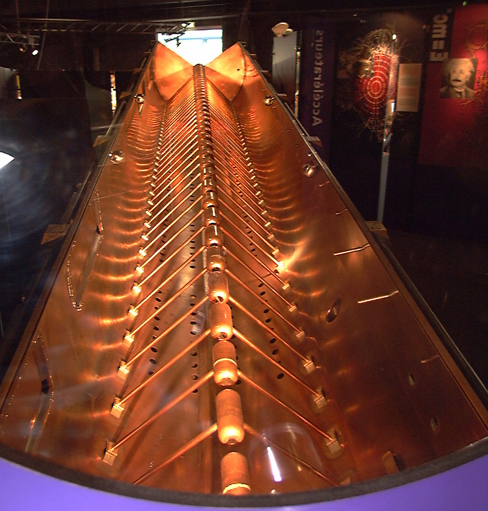
($x$ in the animation corresponds to our $s$)
Drift tube linear accelerators (DTLs) consist of many subsequent drift tubes between which the fields oscillate
- distance between two accelerating gaps depends on particle velocity $\beta c$
$\implies$ synchronism condition for linacs $\leftrightarrow$ length of drift tubes - maximum energy reach scales with length of linac and rf accelerating gradient ($\approx$ MV/m)
- RF structure at high frequency provides micro-bunches
Part II: Longitudinal Drift
Longitudinal phase space: $({\color{red}{z}}, \delta)$Drifting on a non-curved trajectory
The synchronous particle moves with $s=\beta ct$ along the reference path.
The longitudinal offset of a given real particle $z$ relates to its distance at $s$ compared to the synchronous particle after a given time $t$:
$$z=s - \beta c t$$
Consider a drift length $L_d$ (without any fields present) traversed by the synchronous particle in $T_d=\cfrac{L_d}{\beta c}$. A real particle would arrive with $T_d+\Delta t$:
$$z=L-\beta c(T_d+\Delta t)=-\beta c \Delta t$$
On a straight reference trajectory, the delay $\Delta t$ directly relates to the change in speed $\Delta\beta$:
$$\cfrac{\Delta t}{T_d} = -\cfrac{\Delta \beta}{\beta}$$
$$\implies z=-\beta c \Delta t = T_d c \Delta \beta = L_d \frac{\Delta \beta}{\beta}$$
This $\Delta\beta$ corresponds to a momentum deviation $\Delta p/p_0=\delta$ of the real particle. Using the total momentum definition and $\gamma\equiv 1/\sqrt{1-\beta^2}$,
$$p = \beta\gamma m_0 c \implies \underbrace{\frac{\Delta p}{p_0}}\limits_{\equiv \delta} = \frac{\Delta\beta}{\beta} + \underbrace{\frac{\Delta\gamma}{\gamma}}\limits_{\left(\gamma^2-1\right)\Delta\beta/\beta} = \gamma^2\cdot \frac{\Delta\beta}{\beta}$$
which yields the update relation for the offset $z$ after a longitudinal drift according to a momentum deviation $\delta$:
Linacs: Longitudinal Update Map I
The energy gain in the rf cavity,
$$\Delta E|_\text{after} = \Delta E|_\text{before} + q V\cdot \left(\sin\left(\varphi_s - \frac{\omega_\text{rf}z}{\beta c}\right) - \sin(\varphi_s)\right) \quad ,$$
and the longitudinal drifting, $z|_\text{after} = z|_\text{before}+\cfrac{L_d}{\gamma^2}\,\delta$, form the discrete longitudinal update map or linac tracking equations (in absence of curvature (dipoles) and other energy loss terms such as synchrotron radiation).
With $\delta = \frac{\Delta p}{p_0} = \frac{1}{p_0}\cdot \frac{\Delta E}{\beta c}$, we can express them in $(z,\delta)$ phase space coordinates in absence of acceleration ($\varphi_s=0$):
$$\delta_{n+1} = \delta_n + \cfrac{q V}{\beta c p_0}\cdot\sin\left(\varphi_s - \cfrac{\omega_\text{rf}z_{n+1}}{\beta c}\right) \quad .$$
Linacs: Longitudinal Update Map II
With acceleration, $p_0$ changes, and it is more convenient to use $(\Delta t, \Delta E)$ or $(z,\Delta p)$ as phase space coordinates.
$$\begin{cases}\, z_{n+1} &= z_n + \cfrac{L_d}{\gamma_n^2} \left(\cfrac{\Delta p}{p_0}\right)_n \\ (\Delta p)_{n+1} &= (\Delta p)_n + \cfrac{q V}{(\beta c)_n}\cdot\left(\sin\left(\varphi_s - \cfrac{\omega_\text{rf}z_{n+1}}{\beta c}\right) - \sin(\varphi_s)\right) \end{cases}$$
with the synchronous phase $\varphi_s$ determined by $(\delta p_0)_{\text{turn}} = \frac{q V}{\beta c}\,\sin\bigl(\varphi_s\bigr)$.
Part III: Tracking Example in CERN LINAC4
Longitudinal particle tracking in a linear accelerator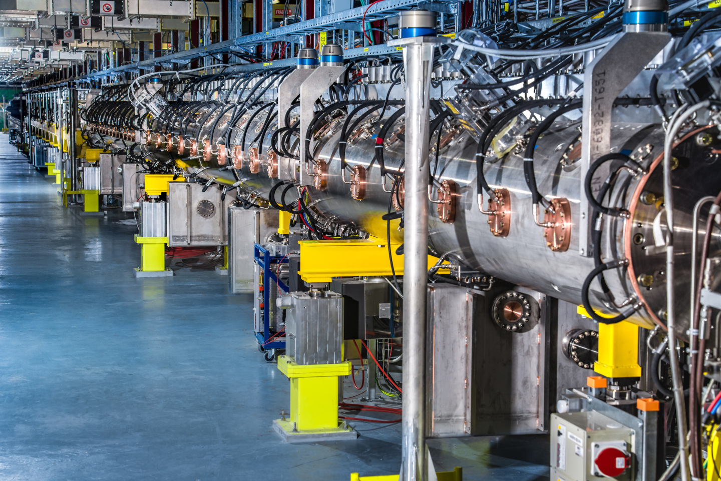
LINAC4 Features
- 86m long staged linear accelerator delivering H${}^-$ ion beams at 160 MeV
- Accelerates from the source to the first synchrotron, the PS Booster
- Operates since 2020 as first stage to produce beams for the LHC, key element of LHC High Luminosity Upgrade
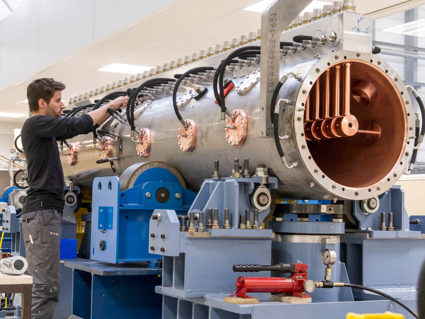
The 19m long DTL section has 3 tanks with a total of 111 drift tubes:
- accelerate from $E_\text{kin}=$ 3 MeV to 50 MeV
- RF frequency at $f_\text{RF}=$ 352 MHz
- RF voltage per gap $V\approx$ 0.5 MV/m
- synchronous phase $\varphi_s\approx$ 70 deg
Gap voltage and synchronous phase (Linac convention)
The DTL corresponds to the first 111 data points (see red label):
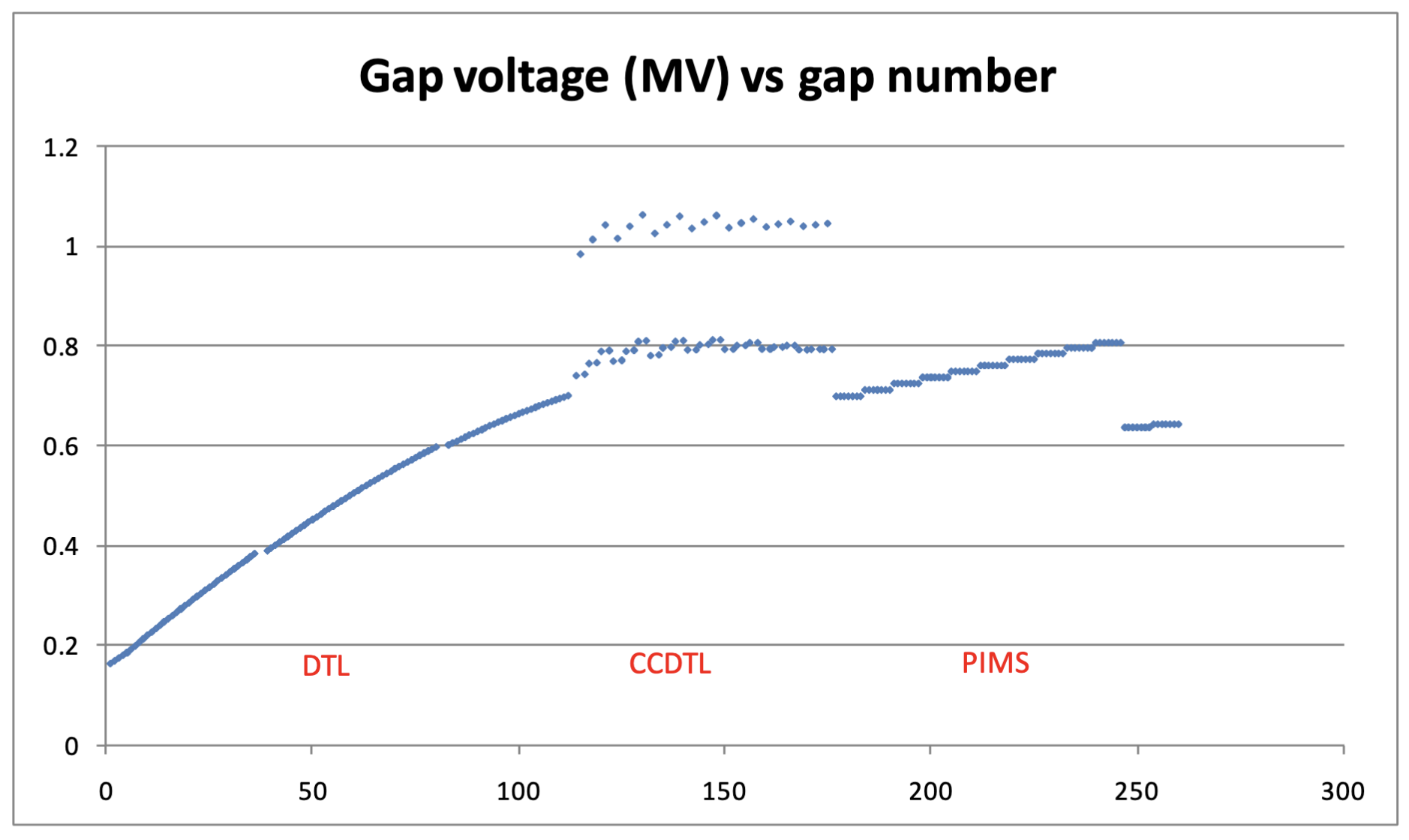
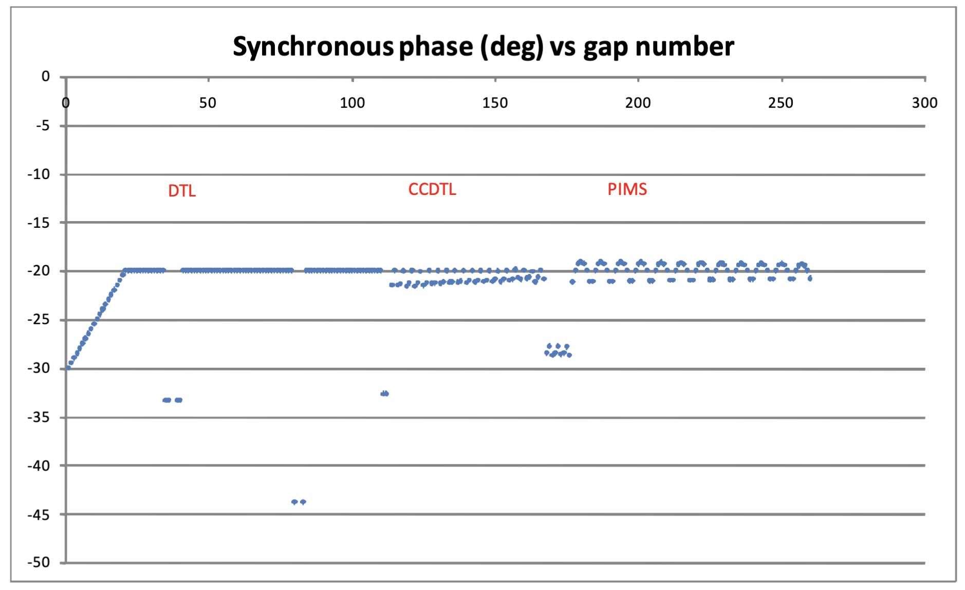
NB: linacs often use the cosine phase convention, $\Delta W_0 = q V\cdot\cos(\varphi_s)$, while we stick to $\Delta W_0 = q V\cdot\sin(\varphi_s)$ throughout this course.
$\implies$ translate y-axis of right plot from $\varphi$ to $\varphi+90\deg$ for our convention!
figures by A.M. Lombardi et al.
Simplistic Tracking Example
Let us track a bunch of H${}^-$ particles through the DTL!
First compute the initial Lorentz factor $\gamma$ at the start of the DTL – remember to use SI units throughout:
from scipy.constants import m_p, e, c

charge = -e #fill me
mass = m_p #fill me

gamma_ini = 1 + 1/(mass * c**2) * 3e6 * e #fill me
gamma_ini
1.0031973667700465
Some convenience functions to compute the speed β and the relativistic Lorentz factor γ:
def beta(gamma):
    '''Speed β in units of c from relativistic Lorentz factor γ.'''
    return np.sqrt(1 - gamma**-2)

def gamma(p):
    '''Relativistic Lorentz factor γ from total momentum p.'''
    return np.sqrt(1 + (p / (mass * c))**2)
What is the RF wavelength of LINAC4?
lambda_rf = c / 352e6 #fill me
lambda_rf
0.8516831193181819
How long would you expect a bunch of particles to be?
bunch_length = 1e-3 #fill me
bunch_length
0.001
Fill in the missing parameters to define the Linac machine object:
class Machine(object):
    # units: SI, phi_s in rad:
    gamma_ref = gamma_ini #fill me
    total_length = 19. #fill me
    n_drifts = 111 #fill me
    voltage = 0.5e6 #fill me
    frequency = 352e6 #fill me
    phi_s = -70 * np.pi/180

    def p0(self):
        '''Momentum of synchronous particle.'''
        return self.gamma_ref * beta(self.gamma_ref) * mass * c

    def update_gamma_ref(self):
        '''Advance the energy of the synchronous particle
        according to the synchronous phase by one cavity kick.
        '''
        deltap_per_turn = charge * self.voltage / (
            beta(self.gamma_ref) * c) * np.sin(self.phi_s)
        new_p0 = self.p0() + deltap_per_turn
        self.gamma_ref = gamma(new_p0)

    def reset(self):
        self.gamma_ref = gamma_ini
This is our tracking function which advances the particles by one drift tube and a gap:
def track_one_tube(z_n, deltap_n, machine):
    m = machine
    Ld = m.total_length / m.n_drifts
    # drift
    z_n1 = z_n - Ld / m.gamma_ref**2 * deltap_n / m.p0()
    # rf kick
    amplitude = charge * m.voltage / (beta(gamma(m.p0())) * c)
    phi = m.phi_s - 2 * np.pi * m.frequency * z_n1 / (beta(gamma(m.p0())) * c)

    deltap_n1 = deltap_n + amplitude * (np.sin(phi) - np.sin(m.phi_s))
    m.update_gamma_ref()
    return z_n1, deltap_n1
The Machine instance will keep track of the reference energy during the tracking by calling update_gamma_ref() once per rf cavity kick:
m = Machine()
Particles are tracked by their two longitudinal coordinates $(z, \Delta p)$. The initial values are stored in z_ini and deltap_ini as numpy.arrays. These should have N entries for $N$ particles.
(You may use numpy helper functions such as np.linspace or np.arange for convenient initialisation!)
z_ini = np.linspace(-bunch_length/2, bunch_length/2, 50)
deltap_ini = np.zeros_like(z_ini)

N = len(z_ini)
assert (N == len(deltap_ini))
To store the coordinate values during tracking, prepare some n_drifts long 2D arrays with N entries per turn:
z = np.zeros((m.n_drifts, N), dtype=np.float64)
deltap = np.zeros_like(z)

z[0] = z_ini
deltap[0] = deltap_ini
We would also like to store the reference beta for each turn:
betas = np.zeros(m.n_drifts, dtype=np.float64)
betas[0] = beta(m.gamma_ref)
Tracking Loop!
Let's go, here's the tracking loop along the DTL!
m.reset()

for i_turn in range(1, m.n_drifts):
    z[i_turn], deltap[i_turn] = track_one_tube(z[i_turn - 1], deltap[i_turn - 1], m)
    betas[i_turn] = beta(m.gamma_ref)
Check: did we reach the (correct) final energy?
"Ekin = {:.2e} eV".format((m.gamma_ref - 1) * mass * c**2 / e)
'Ekin = 5.50e+07 eV'
Change of speed along DTL
plt.plot(betas)
plt.xlabel('Turns')
plt.ylabel(r'$\beta$');

Phase space portrait of particles along DTL
plt.scatter(z, deltap / m.p0(), marker='.', s=0.5)
plt.xlabel('$z$ [m]')
plt.ylabel('$\Delta p/p_0$')
Text(0, 0.5, '$\\Delta p/p_0$')

Questions about Longitudinal Dynamics Linac Model
- Which parameter do we need to adjust to accelerate to $\approx$ 50 MeV?
(Given the sign of the H${}^-$ particle charge, in which direction do you change that parameter?)
- What type of particle motion are we observing?
- What happens if you increase the bunch length significantly (approaching the RF wavelength)?
- What could you do to further increase the acceleration rate? Observe what happens to the stability of the particles if you increase the synchronous phase $\varphi_s$?
- Which part of this Linac longitudinal dynamics model is overly simplistic?
Summary
- Lorentz force, longitudinal $E_z$ field component only means to accelerate
- transit-time factor
- energy gain in rf cavity: synchronous particle and real particles
- linacs
- phase focusing and stability $=$ bunching
- longitudinal particle tracking equations for linacs
Some considerations on rf cavity modelling for reference
Approximation #1: Velocity Change
A priori, energy gain is associated with particle velocity change, i.e. exact $T$ depends on $d\beta$ during passage through rf cavity.
For medium-energy linacs and synchrotrons, effect of velocity change can be neglected to determine energy gain ($\Delta W\propto\Delta\gamma$):
$$\frac{d\beta}{\beta} = \frac{1}{\beta^2\gamma^2} \cdot \frac{d\gamma}{\gamma}$$
$\implies$ two scenarios where approximation of $T$ independence of $\Delta\beta$ applies:
$$\begin{cases}\, \gamma \gg 1 &:\quad\text{particle is already ultra-relativistic} \\[0.3em] \Delta\gamma \ll \beta\gamma &:\quad\text{cavity energy gain much smaller than particle momentum} \end{cases}$$
Simple Example for $T$
Consider uniform standing wave with $E_{z,0}(s)=V_0/g=\mathrm{const}$ across gap width $g$ (zero field outside), at crest of rf wave, i.e. $\varphi_s=\pi/2$:
$$E_z(s, t) = \frac{V_0}{g} \,\cos(\omega_{\text{rf}}\,t)$$
The synchronous particle travels along $s=\beta c t$ (assuming constant $v=\beta c$) and picks up an actual maximum energy gain
$$\implies \Delta W = \cfrac{q V_0}{g}\int\limits_{-g/2}^{+g/2} ds\cdot \cos\left(\cfrac{\omega_{\text{rf}}\,s}{\beta c}\right)$$
and the transit-time factor becomes:
$$T = \left| \cfrac{\sin\left(\cfrac{\omega_\text{rf} g}{2\beta c}\right)}{\cfrac{\omega_{\text{rf}} g}{2\beta c}} \right| \quad \implies\quad T\rightarrow 1 \Leftrightarrow \begin{cases}\, g \rightarrow 0 \\ \omega_{\text{rf}} \rightarrow 0 \\ \beta c \rightarrow \infty \end{cases}$$
$\implies$ reduction in effective energy gain ($T<1$) is mostly relevant for low-energy protons and ions!
Earnshaw's Theorem
S. Earnshaw (1839), Trans. Camb. Phil. Soc. 7 97
$\implies$ application to rf accelerators: always one direction in 3D which is defocused!
Approximation #2: Transverse Defocusing
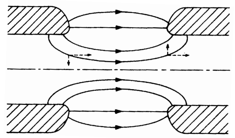
Real $\mathbf{E}$ field across gap in rf cavities has transverse component when off axis, classical regime:
- focusing at entry
- defocusing at exit
$\implies$ DC field leads to net focusing effect (due to gain in longitudinal momentum), but AC field in case of stable longitudinal motion: net defocusing effect (rise in voltage during passage)
$\implies$ typically very weak vs. quadrupole fields and, in synchrotron models, often neglected