Numerical Methods in Accelerator Physics
Demo lecture: phase-space tomography
Notebook lecture by Dr. Adrian Oeftiger $\nearrow$
at TU Darmstadt etit, Fachbereichsrats-Sitzung, on 27.09.2022.
Run this notebook online:
![]()
Also find this lecture rendered on github $\nearrow$ along with the source repository $\nearrow$:
https://github.com/aoeftiger/TUDa-demo-lecture-tomo
Tomographic Reconstruction
"Tomography": imaging via sectioning
Origins: mathematician J. Radon (AUT)
- 1917: "On the determination of functions from their integrals along certain manifolds"
- inverse problem
- Fourier slice theorem: any 2D (3D) object can be reconstructed from infinite set of 1D (2D) projections


Many Applications
- medical: CT scan in hospitals (computed tomography)
- 1979 Nobel price in Medicine:
first CT scanner by Sir G.N. Hounsfield
- 1979 Nobel price in Medicine:
- material science
- airport security
- accelerator physics
- ...
Projection Integral or Radon Transform $\mathcal{R}_\theta(p)$
$$\require{color} \mathcal{R}_\theta(p)\, f = \int dx\int dy~ f(x, y) \,\underbrace{\delta(x\,\cos \theta+y\,\sin\theta-p)}\limits_{\color{red}\text{projection slice}}$$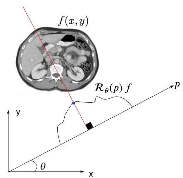
image source: @docmilanfar, Twitter
# imports
from talksetup import *
%matplotlib inline

from skimage.transform import radon, iradon
from PIL import Image
Load sample image for the tomography:
data = ~np.array(Image.open('etit_logo.png').convert('1', dither=False))

plt.imshow(data, cmap='binary')
<matplotlib.image.AxesImage at 0x7f7698e27ba8>

Compute the Radon transform at an angle of 0 deg and 90 deg:
Rf_0 = radon(data, [0], circle=False).astype(float)
Rf_90 = radon(data, [90], circle=False).astype(float)

plt.plot(Rf_0, label='0 deg')
plt.plot(Rf_90, label='90 deg')
plt.legend()
plt.xlabel('$p$')
plt.ylabel(r'$\mathcal{R}_{\theta}(p)f$');

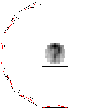
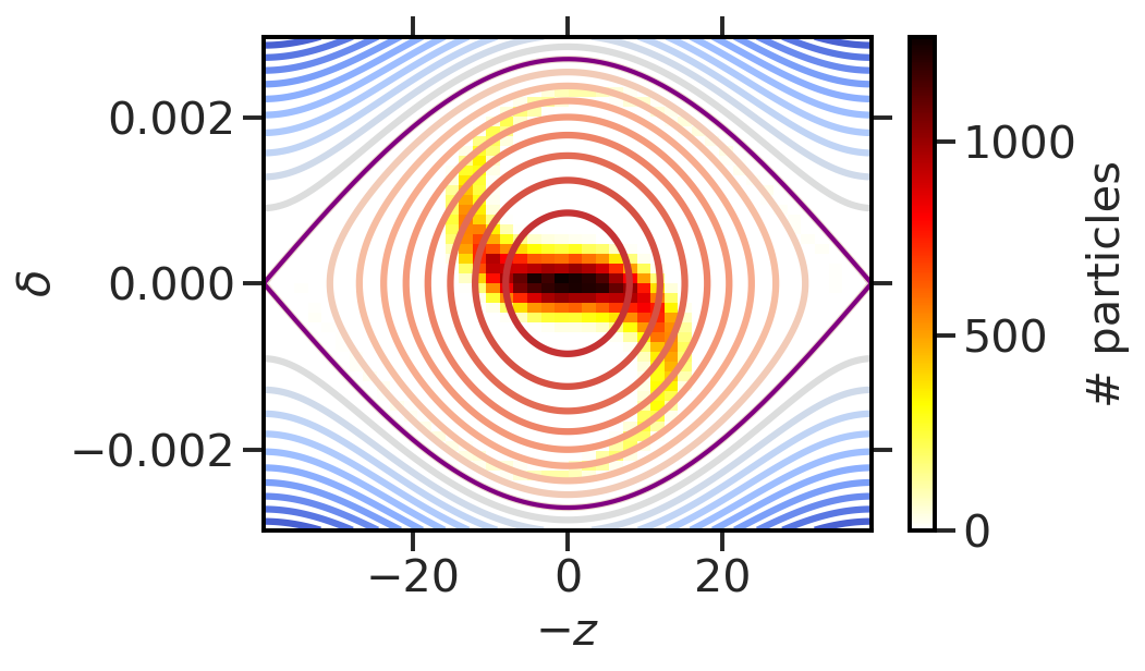
Reconstruction Principle
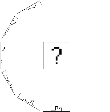
images source: CERN tomography website
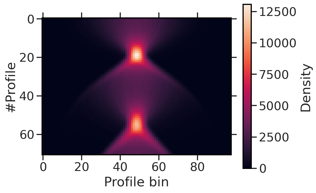
projection (measurement) $\implies$ back-projection (reconstruction)
(Require $ N_{meas} \gtrsim \pi\cdot\frac{\text{total diameter}}{\text{pixel size}}$)
# parameters
N = max(data.shape)
ANG = 180
VIEW = 180
THETA = np.linspace(0, ANG, VIEW, endpoint=False)
# definitions of matrix transforms
A = lambda x: radon(x, THETA, circle=False).astype(float)
AT = lambda y: iradon(y, THETA, circle=False, filter=None,
                      output_size=N).astype(float) * 2 * len(THETA) / np.pi
AINV = lambda y: iradon(y, THETA, circle=False, output_size=N).astype(float)
proj = A(data)
plt.imshow(proj.T)

plt.gca().set_aspect('auto')
plt.xlabel('Projection location [px]')
plt.ylabel('Rotation angle [deg]')
plt.colorbar(label='Intensity');

fbp = AINV(proj)
plt.figure(figsize=(12, 6))
plt.imshow(fbp, cmap='binary', vmin=0, vmax=1);

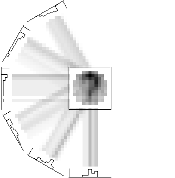
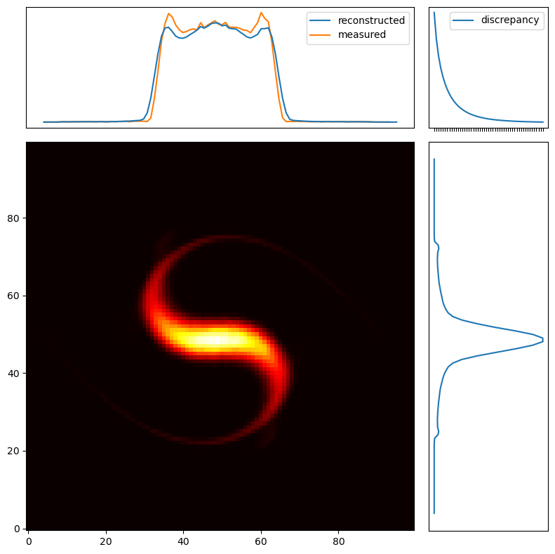
Improved Reconstruction Principle
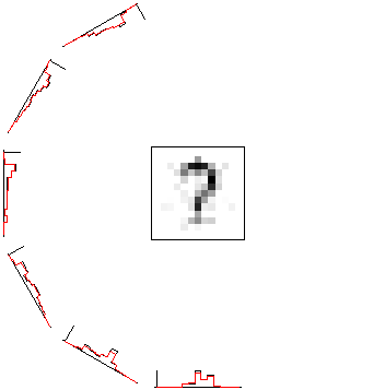
images source: CERN tomography website
projection (measurement) $\implies$ back-projection (reconstruction)
$\stackrel{\text{improve}}{\implies}$ re-projection (red) $\implies$ iteratively reduce discrepancy
Reconstruction Algorithms

Filtered Back-Projection (FBP) vs. Iterative Reconstruction
$\implies$ Iterative algebraic reconstruction technique (ART):
- more computationally expensive than FBP
- more accurate, less artifacts
- can incorporate a priori knowledge
noise = np.random.normal(0, 0.2 * np.max(proj), size=proj.shape)
proj_noise = proj + noise
plt.imshow(proj_noise.T)
plt.gca().set_aspect('auto')
plt.xlabel('Projection location [px]')
plt.ylabel('Rotation angle [deg]')
plt.colorbar(label='Intensity');

fbp_noise = AINV(proj_noise)
plt.imshow(fbp_noise, cmap='binary', vmin=0, vmax=1, interpolation='None');

def ART(A, AT, b, x, mu=1, niter=10):
    ATA = AT(A(np.ones_like(x)))

    for i in tqdm(range(niter)):
        x = x + np.divide(mu * AT(b - A(x)), ATA)

        # nonlinearity: constrain to >= 0 values
        x[x < 0] = 0

        plt.imshow(x, cmap='binary', vmin=0, vmax=1, interpolation='None')
        plt.title("%d / %d" % (i + 1, niter))
        plt.show()

    return x

# initialisation
x0 = np.zeros((N, N))
mu = 1
niter = 10
x_art = ART(A, AT, proj_noise, x0, mu, niter)
0%| | 0/10 [00:00<?, ?it/s]


_, ax = plt.subplots(1, 2, figsize=(10, 5))
plt.subplots_adjust(wspace=0.3)

plt.sca(ax[0])
plt.imshow(fbp_noise, cmap='binary', vmin=0, vmax=1, interpolation='None')
plt.title('FBP')

plt.sca(ax[1])
plt.imshow(x_art, cmap='binary', vmin=0, vmax=1, interpolation='None')
plt.title('ART');

Summary
- Radon transform
- Tomographic reconstruction algorithms:
- filtered back-projection
- iterative: algebraic reconstruction technique
$\implies$ Go ahead, try out the accelerator physics example $\nearrow$
Further literature: Chapter 3 of A. C. Kak and Malcolm Slaney, Principles of Computerized Tomographic Imaging, Society of Industrial and Applied Mathematics, 2001