Numerical Methods in Accelerator Physics

Lecture Series by Dr. Adrian Oeftiger

Guest Lecture by Dr. Michael Schenk

Lecture 12

Run this notebook online!

Interact and run this jupyter notebook online:

via the public mybinder.org service:

via the public gesis.org service:

Also find this lecture rendered as HTML slides on github $\nearrow$ along with the source repository $\nearrow$.

Run this first!

Imports and modules:

from config import (np, plt, print_qtable, Maze, QLearner, plot_q_table, 
                    plot_greedy_policy, tf, e_trajectory,
                    ClassicalDDPG, trainer, plot_training_log, run_correction)
%matplotlib inline

If the progress bar by tqdm (trange) in this document does not work, run this:

!jupyter nbextension enable --py widgetsnbextension

Enabling notebook extension jupyter-js-widgets/extension...
      - Validating: OK

Refresher!

• Bayesian Optimisation (BO) as global optimisation method for black-box functions
• Gaussian Process (GP): statistical surrogate model
• Acquisition Function: guide the optimisation
• BO suitable for optimisation – not for control tasks
• adequate for moderate amount of dimensions (~100)

Today!

1. Introduction to Reinforcement Learning
2. Reinforcement Learning Formalism
3. Q-learning
4. Actor-critic Methods

Disclaimer

• Today's introduction to reinforcement learning (RL) is by no means (mathematically) complete
• Want to give a high-level overview and some first ideas on the subject to hopefully spark your interest :)
• RL is a fascinating field: if you want to learn more, there are some great resources at the end of these slides and on the web

Part I: Introduction to Reinforcement Learning

Machine learning landscape

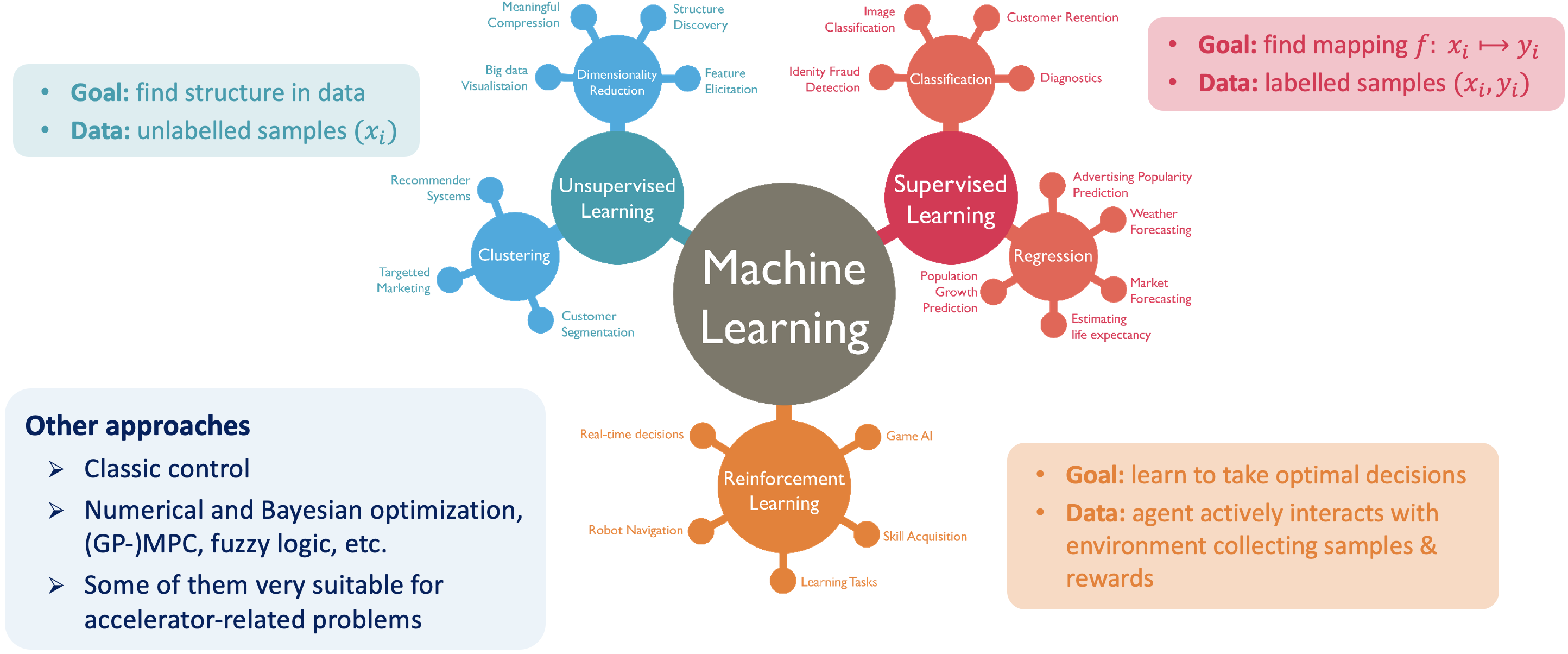
image by GeekStyle

Reinforcement learning examples

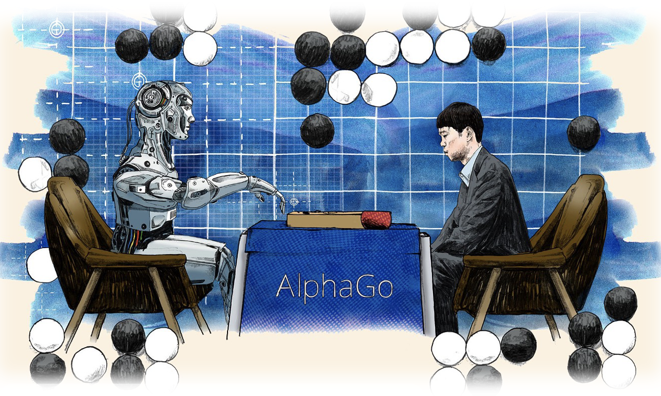
DeepMind, 2015 & 2017: AlphaGo & AlphaZero

• Famous RL success story: agent learns to play the game of Go and beats world champion Lee Sedol
• In case you want to know more: documentary on YouTube

DeepMind AlphaGo

Reinforcement learning examples

OpenAI, 2019: hide-and-seek

• RL agents learning to play hide-and-seek in a multi-agent setting
• Recommend to watch the short video

OpenAI

Reinforcement learning examples

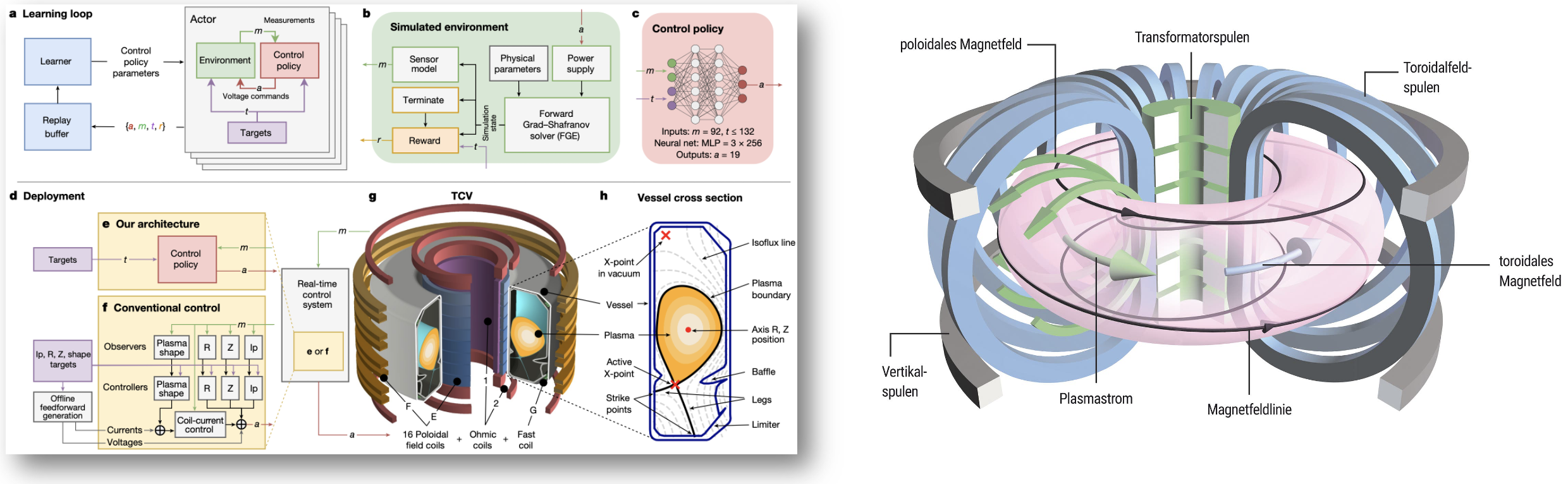
DeepMind & EPFL, 2022: tokamak control

• Shaping and maintaining high-temperature plasma within tokamak vessel is challenging
• Requires high-dimensional, high-frequency, closed-loop control using magnetic actuator coils
• Paper describes RL agent that was successfully trained as a magnetic controller

Paper, EuroFusion

Reinforcement learning examples

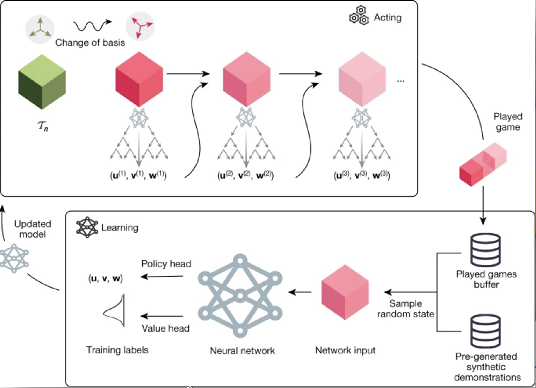
DeepMind, 2022: AlphaTensor

• Improve computational efficiency of matrix multiplication
• RL agent discovered more efficient algorithms than those developed by humans
• Benefits countless fields

Paper

Reinforcement learning examples

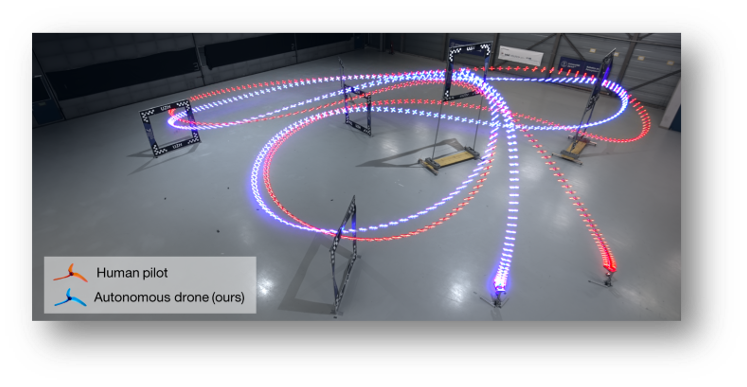
UZH & Intel Labs, 2023: Drone racing

• Training in simulations with mixed-in residual models from real data
• RL agent beats human drone racing champions in real environment

Paper

What is reinforcement learning?

• Application: online optimal control, decision-making tasks
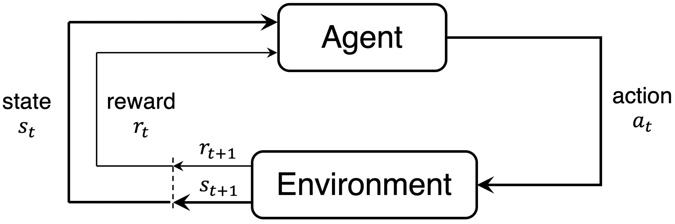
• Trial-and-error learning: for environment in state $s_t$, agent takes action $a_t$ and collects reward $r_t$
• Goal: learn optimal behavior in an environment
  • Behavior: a.k.a. policy $\pi$ - "what action to pick in a given state?"
  • Optimality: maximizing return $G_t = \sum_{k = 0} \gamma^k\,r_{t+k}$ with $\gamma \in (0, 1)$
• Can be solved in various ways: many algorithms exist
• We provide minimal input: reward function, state definition, action space

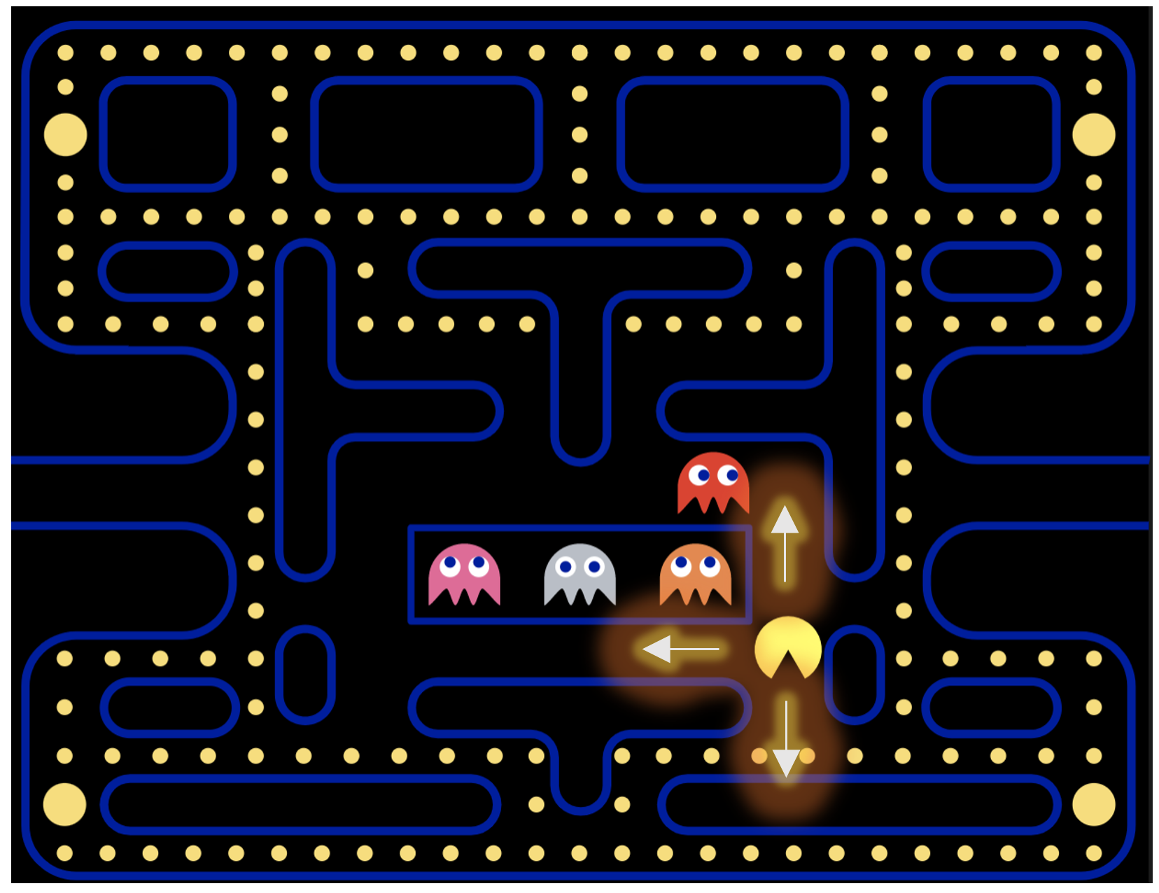
An example: Pacman

• For games it is typically easy to define what the state, actions, and rewards are
  • State: where am I? Where are ghosts, snacks, cookies?
  • Actions: up, down, left, right
  • Reward: food (+), ghosts (-)
  • Return: how much food am I going to eat over time?
  • Policy: based on current state of the screen, should I go up, down, left, or right?

Another example: beam trajectory steering

• Maximize integrated beam on target
  • State: beam position somewhere in the line (continuous variable)
  • Action: increase or decrease dipole kick angle, or strength (continuous variable)
  • Reward: amount of beam on target

Today's lecture

• There are various RL algorithms suitable for different types of tasks

• Often the choice of algorithm depends on whether we deal with discrete or continuous state-action spaces

• We will go through:

  1. Discrete states, discrete actions: Q-learning with a lookup table
  2. Continuous states, discrete actions: Q-learning with a neural network (deep Q-learning or DQN)
  3. Continuous states, continuous actions: actor-critic algorithm $\Rightarrow$ what we typically need to control accelerator systems ...

Our environment

• A small grid maze
• There are fires and a target field
• A player, or agent has to navigate through and find the target field

env = Maze(height=3, width=5)
env.plot(title='Initial state');

# Take some actions
env.plot(title='Initial state')
env.step(action='up')
env.plot()
env.step(action='right')
env.plot();

RL definitions

• State: player / agent position ( x ) whose coordinates are defined by a tuple $(x, y)$
• Action: 'up', 'down', 'left', 'right'
• Reward: every action comes with a reward, depending on the new state we end up in
  • Taking a step into an empty field: -1
  • Bumping into walls: -5
  • Going through fire: -10
  • Reaching the goal: +30

RL is about taking the best decisions ...

• Obviously there are better and worse trajectories to reach the target. "Better" and "worse" refer to how much reward we can collect along the way.
• We will get back to that

Exercise 1

Using the reward definitions from the previous slide, try to calculate the cumulative rewards for the trajectories shown below. Can you tell which of the paths are equally good / bad?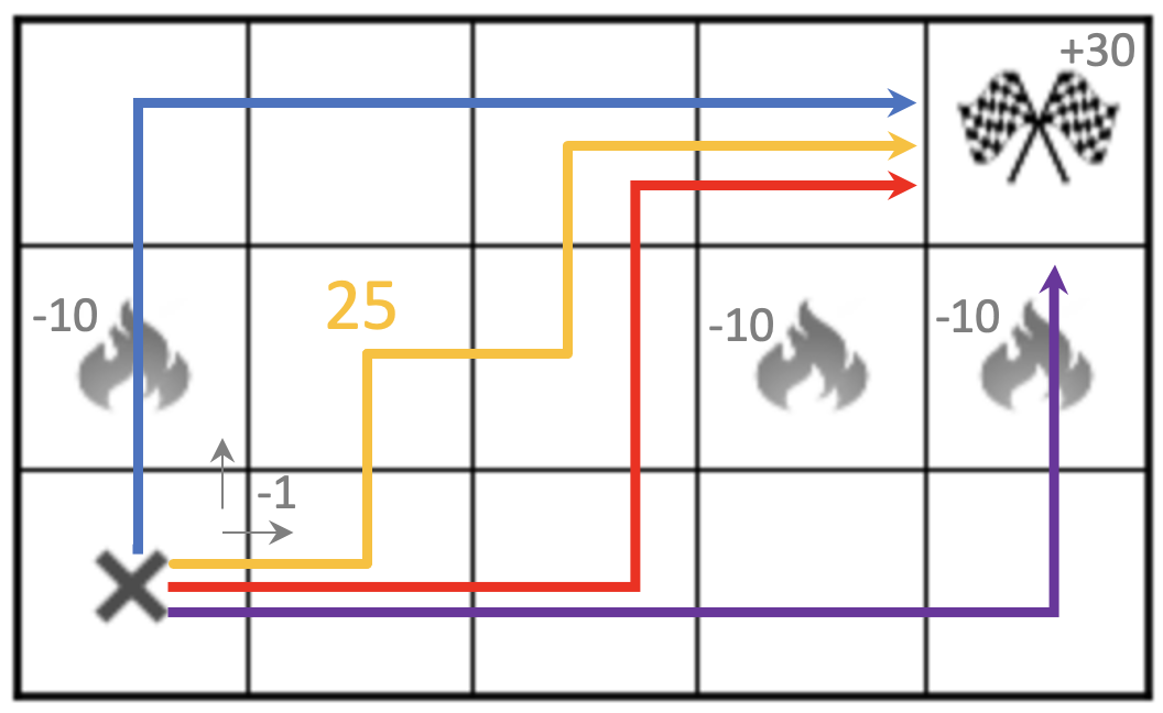

Part II: Reinforcement Learning Formalism

Markov process

• A memoryless random process consisting of a set of states $S$ and state transition probabilities
• The state should possess the Markov property:
  • At every time $t$, the future evolution of the environment depends only on the information contained in the current state $s_t$, but not on the history of past states $s_{t-1}, s_{t-2}, ...$ (memorylessness)
  • In other words: $P(s_{t+1} | s_t) = P(s_{t+1} | s_{t}, s_{t-1}, ..., s_0)$
• Examples:
  • Chess: the positions of the figures on the board fully define the state. There are many ways to reach the specific state, but it does not matter for making the next move nor for the future evolution of the game.
  • Flight of a cannonball: state given by its current position and velocity vector provides enough information to predict the future. (non-Markov: if state only contains the current position, but not the velocity)

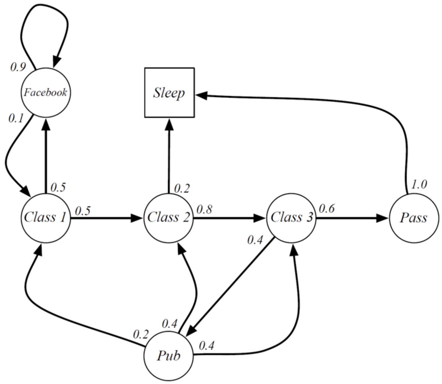
image by D. Silver - Lecture on RL

$S = \{\text{Class 1, Class 2, Class 3, Facebook, Pub, Pass, Sleep}\}$
Note that "Sleep" is also called a terminal state, because once in it we will never leave it.

Markov reward process

• A Markov process that has in addition a reward function and a discount factor $\gamma \in [0, 1]$
• Return $G_t$: sum of discounted future rewards

$$G_t = \sum_k \gamma^k \, r_{t+k}$$

• $\gamma$ controls the relative importance of immediate vs future rewards
  • $\gamma \rightarrow 0$: we only care about immediate rewards
  • $\gamma \rightarrow 1$: we care about rewards far in the future

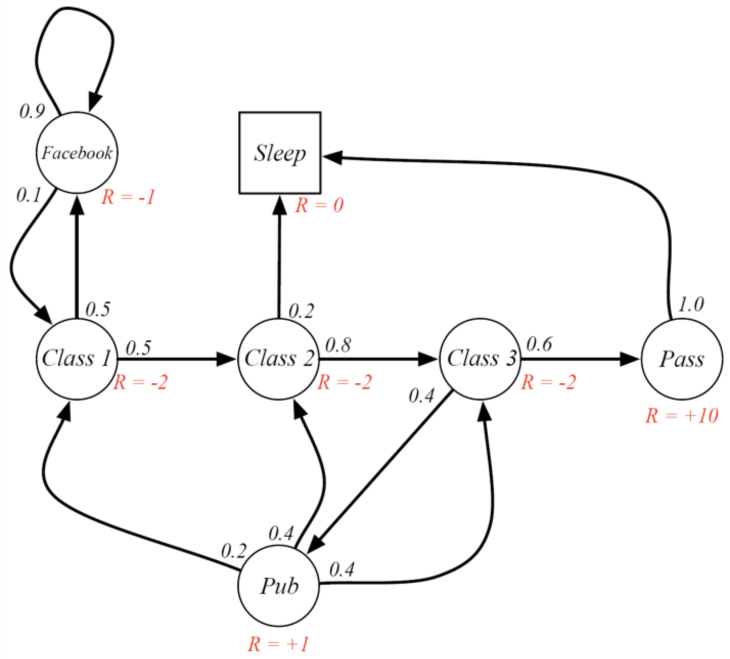
image by D. Silver - Lecture on RL

• Example: C1 $\rightarrow$ C2 $\rightarrow$ C3 $\rightarrow$ Pass $\rightarrow$ Sleep

$\Rightarrow$ Return: $G_0 = (-2) + 0.5 * (-2) + 0.5^2 (-2) + (+10) * 0.5^3 = -2.25$ (with $\gamma = 0.5$)

Markov decision process (MDP)

• Extend Markov reward process by adding decision making: set of possible actions $A$ (= action space)

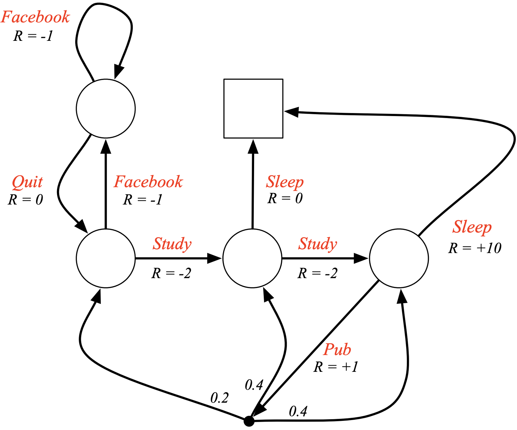
image by D. Silver - Lecture on RL

N.B.: stochastic state transitions are still allowed (if we decide to go to the Pub, anything can happen).
Today we will work with fully deterministic MDPs only.

• Episodic MDP

  • Each episode ends in a terminal state
  • Return $G_t$ is the sum of discounted rewards collected from time $t$ till end of episode
  • Episodes are independent

• Continuous MDP

  • Continues indefinitely: has no terminal states
  • Very important that discount factor $\gamma < 1$ to avoid infinite returns
  • Also known as infinite horizon MDP

Policy $\pi$

• The policy defines the decision making or behavior of the agent
• It is a probability distribution over the state-action space. You can also think of it as a mapping that assigns to each state-action pair $(s, a)$ a probability

$$\pi: S \times A \rightarrow [0, 1]$$

• $S$ and $A$ are the state and action spaces, respectively
  • For our maze: $S = \{[0, 0], [0, 1], ..., [\text{width}-1, \text{height}-1]\}$ and $A = \{\text{'up', 'down', 'left', 'right'}\}$.

Exercise 2

Let's get back to the maze! For now we do not care about optimal decisions. Instead, try to implement a random policy, i.e. every action $a \in \{\text{'up', 'down', 'left', 'right'}\}$ is picked with equal probability no matter what state the agent is in.

a) Initialize a Maze with height=3, width=2 and complete the all_actions list.

b) Look at every step of the output: is the movement of the agent ( x ) and the rewards obtained consistent with your expectations?

c) Change the random number seed, rerun and observe.

np.random.seed(123457)

env = Maze(height=3, width=2) # FILL HERE)
env.plot(title='Initial state')

all_actions = ['up', 'down', 'left', 'right'] # ... FILL HERE]

done = False
while not done:
    action = np.random.choice(all_actions)
    state, action, reward, new_state, done = env.step(action)
    env.plot();

RL objective

• Find optimal behavior in a given environment: in every state we want the agent to take the best action
• This is also known as the optimal policy $\pi^*$
• Formally, $\pi^*$ maximizes the return $G_t = \sum_k \gamma^k \, r_{t+k}$, i.e. the cumulative sum of discounted future rewards.

• For our maze, RL will solve ...
  • For any given field that we are currently on (= state), what is the action that maximizes the sum of rewards collected over time?
  • Or: from where I stand - how can I reach the target field with the least steps and not going through fires (if possible) ?

RL taxonomy

• There are many different algorithms for finding the optimal policy $\pi^*$

• They all have their pros and cons

  • Often the sample-efficiency is crucial
  • It tells us how many interactions with the environment (= how many data samples) we need to solve the RL problem
  • E.g. for accelerator systems: we want to train the agent with as little beam time as possible as it is very expensive

• Today: we are going to look at Q-learning. It is one of the core ideas of many RL algorithms, such as

  • Deep Q-learning (DQN)
  • Actor-critic methods (DDPG, TD3, SAC)

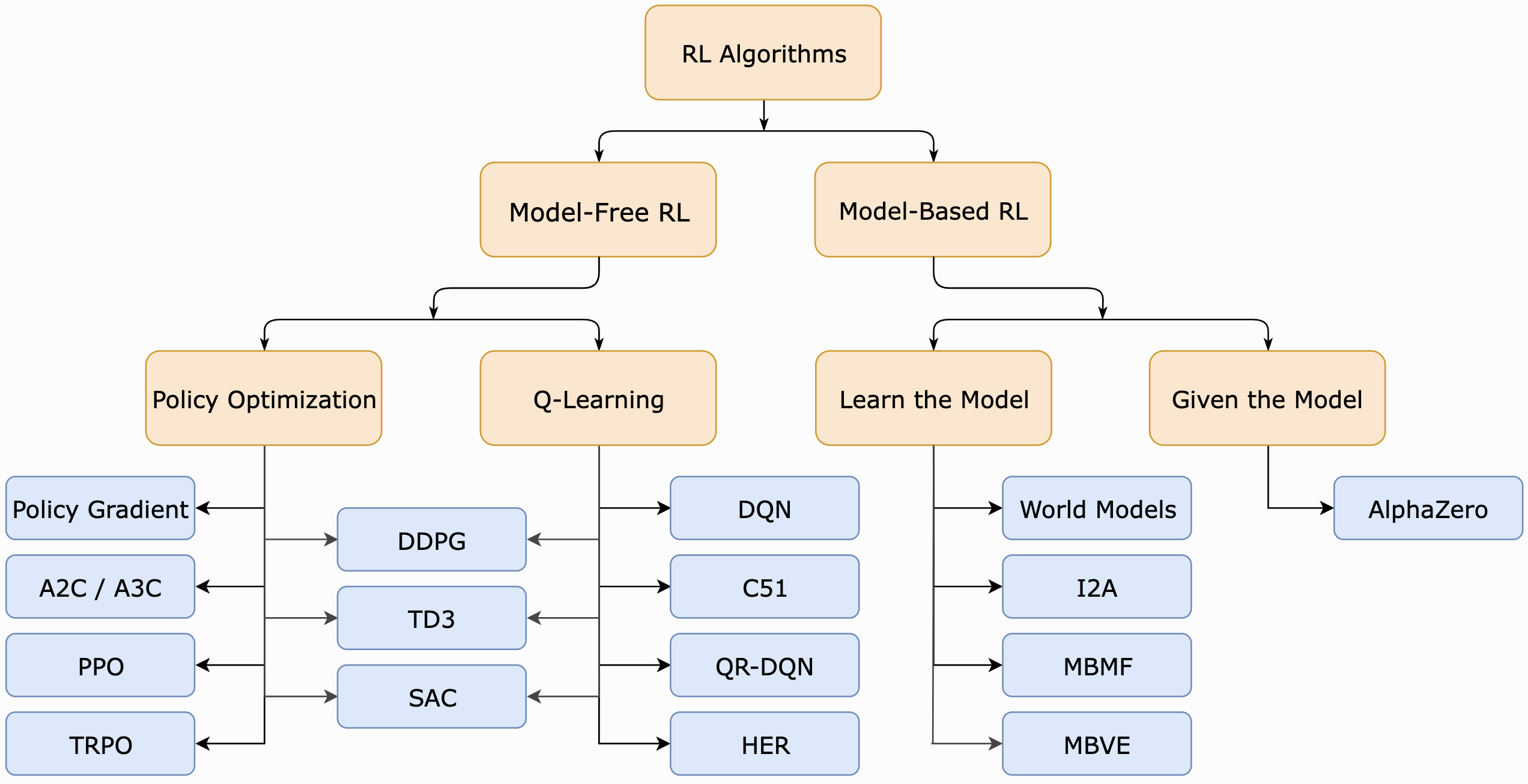
image by Open AI - Spinning Up

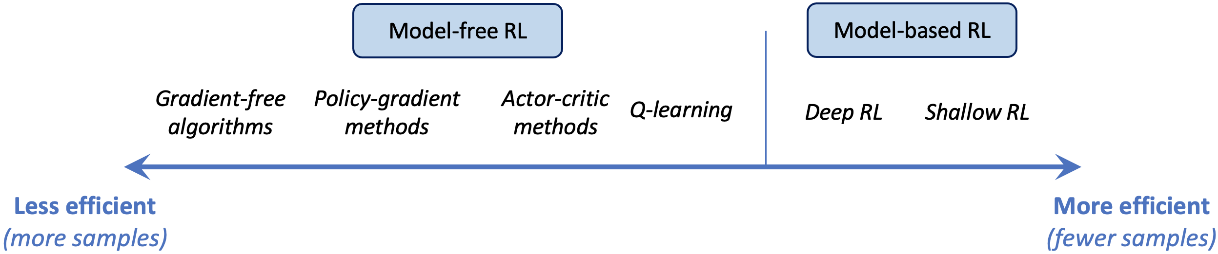
image adapted from S. Levine, "Deep Reinforcement Learning" (lecture)

Intermediate summary

• The goal of RL is to make optimal decisions (take actions) in an environment based on some observables (state)
• Example environments: game, control system (e.g. fusion reactor, tuning accelerator parameters), trading, ...
• The quality of a decision made is quantified by a reward
• Through trial-and-error the RL agent collects rewards and can eventually learn the best behavior (optimal policy $\pi^*$)
• Formally this is described as a Markov decision process (MDP)

Part III: Q-learning

Q-learning

• Employs a state-action value function

$$Q: S \times A \rightarrow \mathbb{R}$$

to solve the RL problem

• The Q-value $Q(s, a)$ characterizes the "quality" of the state-action pair $(s, a)$
  • Quality is measured as the expected return acting according to a certain policy
  $$Q(s, a) = \mathbb{E}[G_t | S_t = s, A_t = a]$$
  • Reminder: $G_t = \sum_k \gamma^k \, r_{t+k}$
  • Q answers: “In a given state, what is the best action to take to maximize return?”

• Temporal difference (TD) learning or learning the Q-function
  • We can write the Q-value of $(s_t, a_t)$ as a sum of immediate reward $r$ plus discounted Q-value of the next state-action pair $(s_{t+1}, a_{t+1})$
  • We are acting greedily, hence the $\text{max}$ operation*

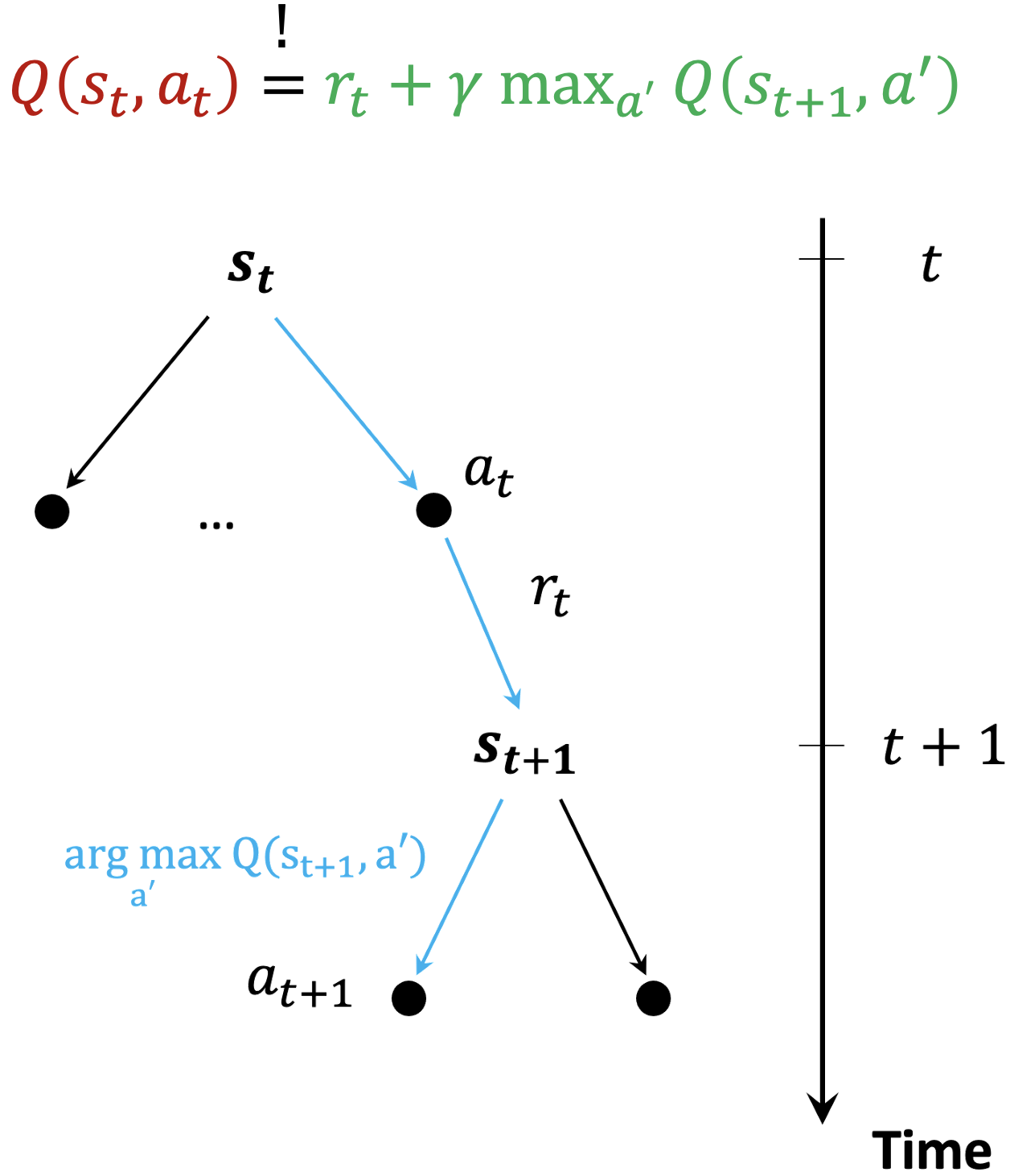
• Temporal difference (TD) rule
  • Q-values are initially unknown / random
  • Learn iteratively following TD update rule using collected interactions with environment

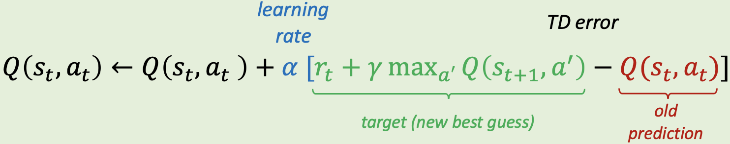
• Use trial-and-error experiences collected by the agent $(s_t, a_t, r_t, s_{t+1})$: state, action, reward, next state.
• This is the core idea of Q-learning and is a result of one of the Bellman equations
• Bootstrapping: update Q-value using target based on estimate $\rightarrow$ a moving target”: training could be unstable, hence double Q-learning

Obtaining the optimal policy

• Once Q-values have converged, it is easy to read off the optimal policy $\pi^*$

$$ \pi^*(s, a) = \left\{ \begin{array}{ll} 1 & \mbox{if } a = \text{argmax}_{a'} \, Q(s, a') \\ 0 & \mbox{otherwise.} \end{array} \right. $$

• This is also known as the greedy policy: it acts greedily in terms of expected return by assigning probability $1$ to the action that maximizes the Q-function.

How to implement Q-learning?

• We need a way to track and update the Q-value for each state-action pair
  • Traditional Q-learning: Q-table
  • Deep Q-learning: neural network

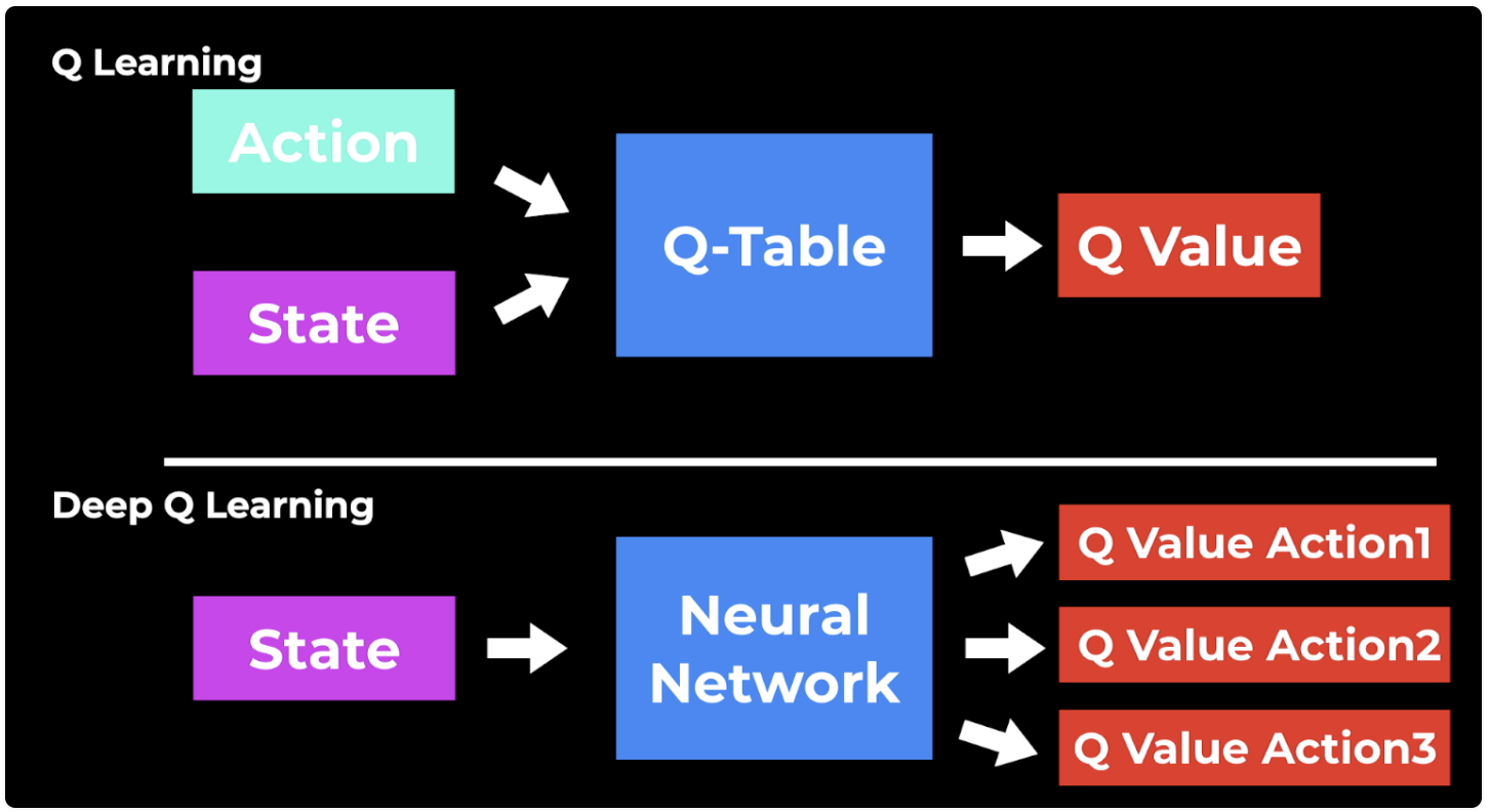
image by AssemblyAI

Some challenges

• Reward engineering
• Definition of the state, which is sometimes only partially observable
• Hyperparameter tuning, making training stable
• Exploration vs exploitation ...

Exploration-exploitation trade-off

• To learn the best policy in the most efficient manner, we need a trade-off between exploration and exploitation.
• We have to ensure that the agent keeps exploring new actions during training and does not just always follow the path that provides the highest expected return
• After all, Q-values might not have converged yet, there may still be better solutions than currently known

image by Berkeley AI course

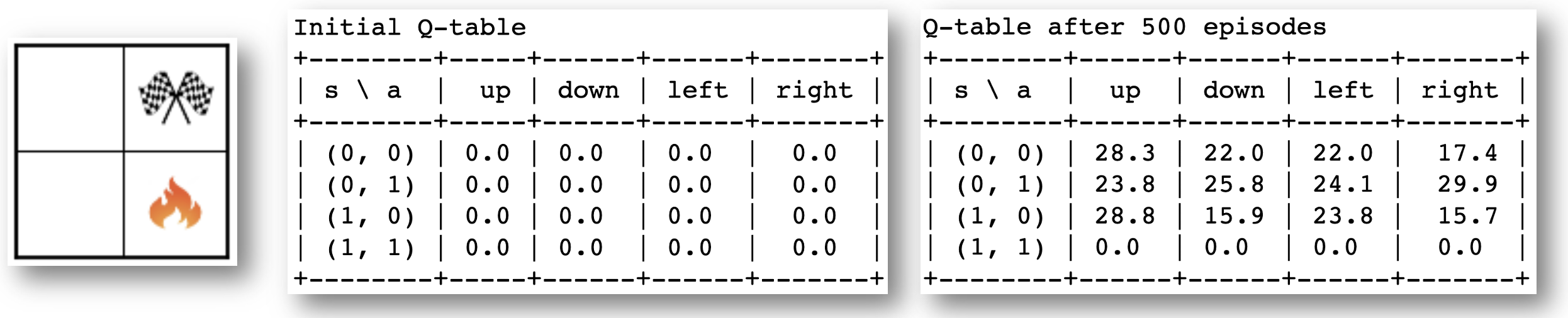
Q-learning with lookup table

• The first Q-learning method we consider is using a lookup table to keep track of the Q-values during training
• First, we initialize all Q-values to 0, then update the values according to the TD rule
• N.B.: this method works only for discrete sets of states and actions

np.random.seed(0)

# Initialize small maze environment
env = Maze(width=2, height=2, fire_positions=[[1, 0]])
_ = env.plot(add_player_position=False)

# Initialize Q-learner with Q-table
qtable_learner = QLearner(env, q_function='table')

print('Initial Q-table')
q_table = qtable_learner.q_func.get_q_table()
print_qtable(q_table)

Initial Q-table
+--------+-----+------+------+-------+
| s \ a  |  up | down | left | right |
+--------+-----+------+------+-------+
| (0, 0) | 0.0 | 0.0  | 0.0  |  0.0  |
| (0, 1) | 0.0 | 0.0  | 0.0  |  0.0  |
| (1, 0) | 0.0 | 0.0  | 0.0  |  0.0  |
| (1, 1) | 0.0 | 0.0  | 0.0  |  0.0  |
+--------+-----+------+------+-------+

qtable_learner.train(200)

print('Q-table after 200 episodes')
q_table = qtable_learner.q_func.get_q_table()
print_qtable(q_table)

  0%|          | 0/200 [00:00<?, ?it/s]

Q-table after 200 episodes
+--------+------+------+------+-------+
| s \ a  |  up  | down | left | right |
+--------+------+------+------+-------+
| (0, 0) | 19.9 | 7.8  | 7.9  |  7.1  |
| (0, 1) | 14.8 | 11.0 | 14.1 |  26.6 |
| (1, 0) | 22.0 | 5.0  | 8.7  |  4.4  |
| (1, 1) | 0.0  | 0.0  | 0.0  |  0.0  |
+--------+------+------+------+-------+

qtable_learner.train(300)

print('Q-table after 500 episodes')
q_table = qtable_learner.q_func.get_q_table()
print_qtable(q_table)

  0%|          | 0/300 [00:00<?, ?it/s]

Q-table after 500 episodes
+--------+------+------+------+-------+
| s \ a  |  up  | down | left | right |
+--------+------+------+------+-------+
| (0, 0) | 28.3 | 22.0 | 22.0 |  17.4 |
| (0, 1) | 23.8 | 25.8 | 24.1 |  29.9 |
| (1, 0) | 28.8 | 15.9 | 23.8 |  15.7 |
| (1, 1) | 0.0  | 0.0  | 0.0  |  0.0  |
+--------+------+------+------+-------+

qtable_learner.plot_training_evolution()

Exercise 3

a) Based on the evolution of the Q-values on the previous slide - would you consider the training to be complete after 500 episodes?

b) Play with the number of episodes in the cell below until you find convergence.

c) Observe that some of the Q-table values converge earlier than others during training. Why could that be?

np.random.seed(0)

env = Maze(width=2, height=2, fire_positions=[[1, 0]])

qtable_learner = QLearner(env, q_function='table')
qtable_learner.train(2000) # FILL HERE)
qtable_learner.plot_training_evolution()

  0%|          | 0/2000 [00:00<?, ?it/s]

Exercise 4

a) Initialize a bigger maze width=4, height=3, with fire_positions=[[2, 1], [2, 2]] and use q_function='table' in the QLearner class. Then train it for 5000 episodes.

b) Once the training is finished, plot the Q-values (you can just execute the cell, it is already complete).
Next to each little arrow there is a number that denotes the Q-value of the corresponding action on that field. The red arrow indicates the action with the highest Q-value.

c) Finally, also plot the (greedy) policy by executing the third cell. Compare it to the Q-value plot to verify that we indeed always pick the action with the highest Q-value. Are there fields where two actions would be equally good (which ones)? Can you confirm that by looking at the Q-values?

# Exercise 4 a)
np.random.seed(123456)

env = Maze(width=4, # FILL HERE,
           height=3, # FILL HERE,
           fire_positions=[[2, 1], [2, 2]]) # FILL HERE)

qtable_learner = QLearner(env, q_function='table') # FILL HERE)
qtable_learner.train(5000) # FILL HERE)

  0%|          | 0/5000 [00:00<?, ?it/s]

# In case the training does not work for you for some reason
# you can reload the qtable from a trained agent from file.
# Don't forget to initialize the env as suggested in the
# exercise ...
# Note that the q evolution history of training is not saved
# and will hence not be displayed when reloading from file.

# qtable_learner.q_func.load_q_table('saved_agents/qtable_ex4.json')

# Exercise 4 b)
q_table = qtable_learner.q_func.get_q_table()
ax = env.plot(add_player_position=False, title=False)
plot_q_table(q_table, env.target_position, env.fire_positions, ax=ax)

# Exercise 4 c)
policy = qtable_learner.q_func.get_greedy_policy()
ax = env.plot(add_player_position=False, title=False)
plot_greedy_policy(policy, env.target_position, env.fire_positions, ax=ax)

Exercise 5 (optional)

a) Using the same maze as above, reduce the punishment of going through fire by setting a fire_reward=-2 (instead of -10) in the environment definition.

b) Retrain the agent. How does the policy change compared to Ex. 4? Can you explain why?

np.random.seed(123456)

# Env definition
env = Maze(width=4, height=3, fire_positions=[[2, 1], [2, 2]], fire_reward=-2) # FILL HERE)
qtable_learner = QLearner(env, q_function='table')
qtable_learner.train(500)

# If you have issues with the training, please comment out the
# line qtable_learner.train(5000) above and reload instead the
# qtable by uncommenting the following line.

# qtable_learner.q_func.load_q_table('saved_agents/qtable_ex5.json')

  0%|          | 0/500 [00:00<?, ?it/s]

# Show Q-values
q_table = qtable_learner.q_func.get_q_table()
ax = env.plot(add_player_position=False, title=False)
plot_q_table(q_table, env.target_position, env.fire_positions, ax=ax)

# Show policy
policy = qtable_learner.q_func.get_greedy_policy()
ax = env.plot(add_player_position=False, title=False)
plot_greedy_policy(policy, env.target_position, env.fire_positions, ax=ax)

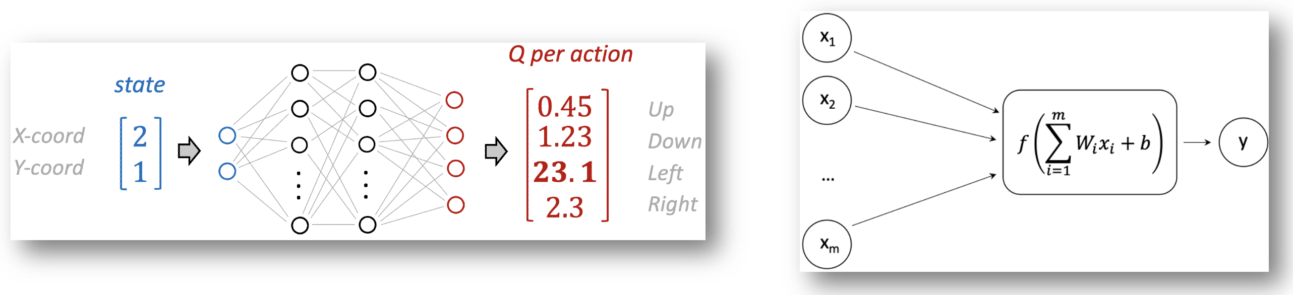
Deep Q-learning (DQN)

• Main idea: replace the Q-table by a simple, feed-forward neural network (Q-net)
• Developed by DeepMind in 2013 to play Atari games (DQN paper)
• A neural network (NN) is a universal function approximator, i.e. a fit model that can approximate any function (in theory)
• The Q-net is a mapping from state to Q-values of all possible actions
• Its parameters a.k.a. weights are adjusted according to the TD rule, like the Q-table

Exercise 6

a) Repeat the same steps as in Ex. 4 for the Q-table learner, but this time using q_function='net' as an argument in the QLearner class. Train it for 1500 episodes. This will take a couple of minutes.

b) Compare the Q-values and policy to the one obtained with Q-table learning. Do you see differences? Why could that be?

tf.keras.utils.set_random_seed(0)

env = Maze(width=4, height=3, fire_positions=[[2, 1], [2, 2]])
qnet_learner = QLearner(env, q_function='net') # FILL HERE)
qnet_learner.train(1500) # FILL HERE)

  0%|          | 0/1500 [00:00<?, ?it/s]

# Again, if you face any issues with model training, please use
# the saved q-net weights of a trained agent by uncommenting
# the following. You can comment the line for training in the
# previous cell.

# qnet_learner.q_func.load_model('saved_agents/qnet_ex6')

q_table = qnet_learner.q_func.get_q_table()
ax = env.plot(add_player_position=False, title=False)
plot_q_table(q_table, env.target_position, env.fire_positions, ax=ax)

policy = qnet_learner.q_func.get_greedy_policy()
ax = env.plot(add_player_position=False, title=False)
plot_greedy_policy(policy, env.target_position, env.fire_positions, ax=ax)

Q-table vs DQN: pros, cons, and limitations

• Q-table

  • Easy to understand and validate

  • Discrete $S$, $A$ spaces only

  • Relatively small $S$, $A$ spaces only

• DQN

  • Big and continuous $S$ possible

  • No need to visit all states during training, because NNs are great interpolators

  • Discrete and relatively small $A$

  • Training may be unstable and harder to verify if we have reached convergence

• Many real-world problems require continuous $S$ and continuous $A$ $\,\,\Rightarrow\,\,$ actor-critic methods

Part IV: Actor-critic Methods

Actor-critic scheme

• Two NNs

• Actor

  • Represents the policy $\pi$ and is a mapping $\pi: S \rightarrow A$
  • For each continuous state, it proposes a continuous action
  • Learns from the critic

• Critic

  • Predicts Q-values and is a mapping $Q: S\times A \rightarrow \mathbb{R}$
  • Evaluates quality of $(s, a)$ pair proposed by actor
  • Feeds back to the actor network: policy gradient rule

N.B.: networks are trained simultaneously

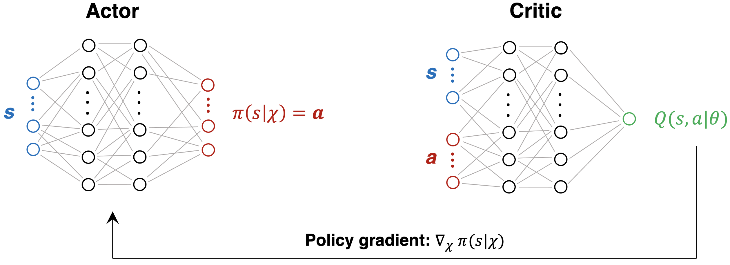
• Critic parameters $\theta$ are updated according to the TD rule, just like in Q-learning
• Actor parameters $\chi$ are updated via policy gradient: for a given state $s$, how does the actor have to adjust its parameters to propose an action $a$ such that $Q(s,a)$ becomes larger?

Application in accelerator physics

• We are going to consider a trajectory steering problem from CERN's AWAKE
• Advanced Proton Driven Plasma Wakefield Acceleration Experiment

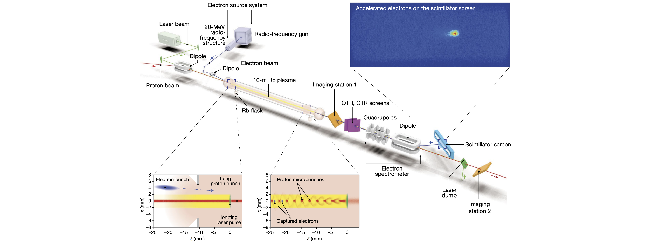
image by AWAKE Collaboration

AWAKE electron beam line

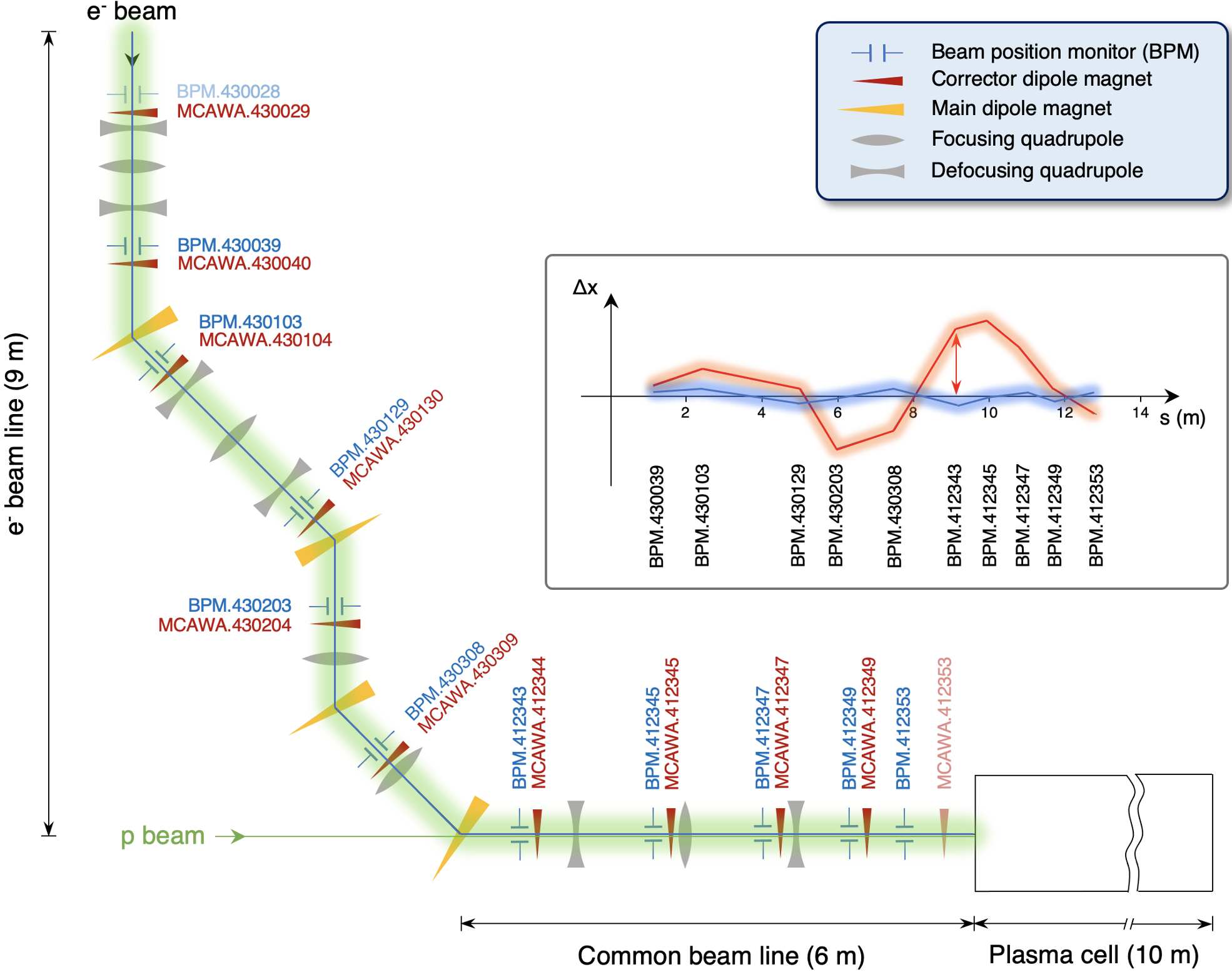
RL task definitions

• Goal: given measured beam positions (= continuous state), find best dipole corrector settings (= continuous actions) to keep beam close to the center of vacuum pipe
• State: 10-d array of beam positions measured along the line
• Action: 10-d array of dipole corrector strengths along the line
• Reward: negative rms of beam offsets wrt. center

Exercise 7

Let's try to train an actor-critic agent on the AWAKE environment! We are using the DDPG (Deep Deterministic Policy Gradient) algorithm. It is one of the most basic actor-critic algorithms and hence also not the most stable one. Some improvements have been implemented in TD3.

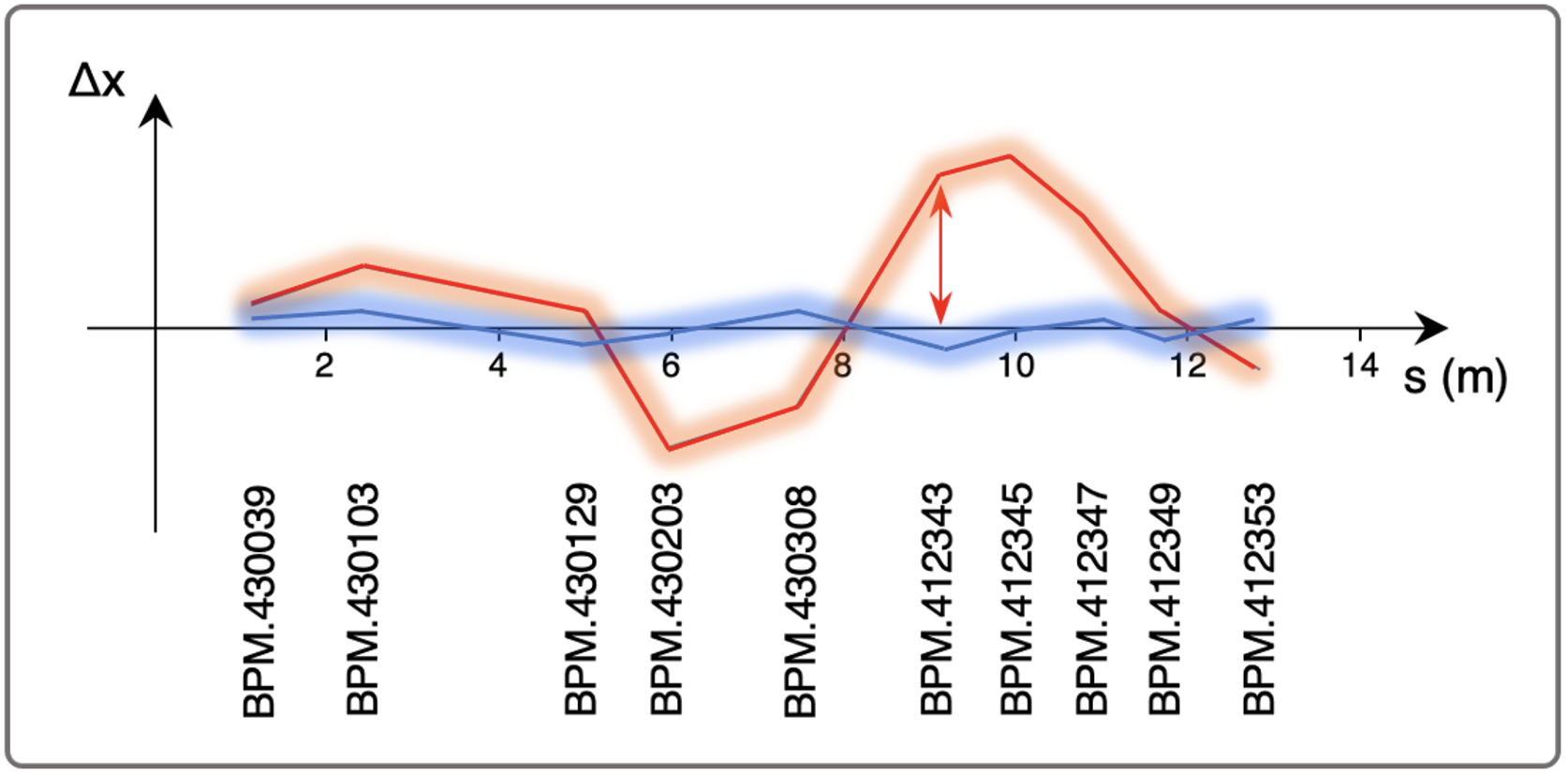
7 a) Run the following cell to initialize the AWAKE simulation environment env and a DDPG instance agent. Then reset the environment to misteer the beam, and plot the trajectory. The plot shows the beam position at the 10 BPMs installed along the electron beam line.

# Exercise 7 a)
tf.keras.utils.set_random_seed(12345)

env = e_trajectory()
agent = ClassicalDDPG(state_space=env.observation_space, action_space=env.action_space)

env.reset(init_outside_threshold=True)
env.plot_trajectory()

7 b) Run the next cell to make a correction to the beam position. Run the cell multiple times and check how the trajectories before and after correction compare. Do you think the RL agent is doing a good job? Why or why not?

# Exercise 7 b)
run_correction(env, agent)

# Exercise 7 b)
run_correction(env, agent)

7 c) Run the next cell to train the RL agent. Can you interpret the output plots showing evolution of agent training? Is the length of training appropriate or should we train with fewer / more steps?

Hints: the output figure shows two axes. The top graph displays the length of each episode over the entire training period (an episode is terminated either when the objective is reached or whenever the agent cannot solve the task after 30 steps). The bottom plot shows the rewards (negative trajectory rms) at the beginning and at the end of an episode. A high negative reward means that the trajectory is badly steered. A reward close to zero on the other hand corresponds to a well-corrected beam trajectory.

# Exercise 7 c)
training_log = trainer(env=env, agent=agent, n_steps=500)

  0%|          | 0/500 [00:00<?, ?it/s]

EPISODE: 0, INITIAL REWARD: -134.26, FINAL REWARD: -73.393, #STEPS: 1.
EPISODE: 50, INITIAL REWARD: -96.326, FINAL REWARD: -49.14, #STEPS: 1.
EPISODE: 100, INITIAL REWARD: -116.591, FINAL REWARD: -38.265, #STEPS: 1.
EPISODE: 150, INITIAL REWARD: -323.567, FINAL REWARD: -75.531, #STEPS: 1.
EPISODE: 200, INITIAL REWARD: -27.811, FINAL REWARD: -60.445, #STEPS: 1.
EPISODE: 250, INITIAL REWARD: -48.02, FINAL REWARD: -57.575, #STEPS: 1.

plot_training_log(env, agent, training_log)

# In case you face any issues with the training of the agent,
# avoid executing the previous cell and use instead the 
# following line to load pre-trained weights.

# agent.load_actor_critic_weights('saved_agents/ddpg_ex7')

7 d) Check a few trajectories before and after correction now using the trained agent (run the cell multiple times). How does the agent perform now?

Note that we are using the DDPG algorithm here which is one of the most basic actor-critic RL algorithms. This is also the reason why the trajectory correction will not always be perfect. There are much improved versions that would train in a shorter time and with better performance (e.g. Twin Delayed DDPG aka TD3).

# Exercise 7 d)
run_correction(env, agent)

Summary

• Reinforcement learning (RL) is concerned with solving decision-making problems and optimizing for best behavior in an environment
• Different algorithms exist with Q-learning being one of the fundamental ones
• Q-learning uses a state-action value function $Q(s,a)$ that estimates the expected return
• $Q(s, a)$ is iteratively learned following the temporal difference rule
• Once converged we can read off the optimal policy by acting greedily with respect to Q
• Q-learning
  • Lookup table: only works for discrete state-action spaces
  • Q-net (neural network): can deal with continuous states
• Actor-critic methods are built on top of Q-learning and use two networks:
  • One for the policy (actor) and one to estimate the Q-values (critic)
  • They can solve tasks with continuous states and actions.

Comprehension questions I

• What do Q-values represent?

• Why does the Q-table only work for discrete state space?

• Why does Q-learning only work for discrete action spaces, both for the Q-table and the Q-net?

• How can you obtain the optimal policy once you know the Q-values?

Comprehension questions II

• Do you have to increase or decrease the discount factor $\gamma$ to put more emphasis on future rewards?

• What is the Markov property? Is it fulfilled for the maze environment? Why, or why not? (hint: think about whether it matters for the future evolution how you ended up on the current field of the maze)

• For the temporal difference learning update, how many different states are involved?

Literature

• R.S. Sutton and A.G. Barto, "Reinforcement learning - an introduction", Book, 2nd edition, 2020.
• S. Levine, Deep Reinforcement Learning, Lecture, UC Berkeley, 2022.
• D. Silver, Reinforcement learning, Lecture, University College London (UCL), 2015.

Python RL libraries

• Stable baselines 3: github, docs
• Gymnasium: github, docs