Numerical Methods in Accelerator Physics

Lecture Series by Dr. Adrian Oeftiger

Lecture 9

Run this notebook online!

Interact and run this jupyter notebook online:

via the public mybinder.org service:

via the public gesis.org service:

Also find this lecture rendered as HTML slides on github $\nearrow$ along with the source repository $\nearrow$.

Run this first!

Imports and modules:

from config import (np, plt, radon, iradon, Image, 
                    tnrange, plot_mp, plot_tomo)
from scipy.constants import m_p, e, c
%matplotlib inline

If the progress bar by tqdm (trange) in this document does not work, run this:

!jupyter nbextension enable --py widgetsnbextension

Enabling notebook extension jupyter-js-widgets/extension...
      - Validating: OK

Refresher!

• Twiss parameters and phase advance from periodic transport matrix
• Betatron matrices and Twiss matrix: 2 representations of identical (stable/bounded) solution to Hill differential equation
• Stability of periodic transport matrices
• Optical / Twiss functions and Dispersion of a FODO cell
• Dipoles generate & quadrupoles focuse dispersion function
• Quadrupole focal length depends on momentum, tune change, chromaticity
• Chromatic tune change in a FODO cell
• Correction of chromaticity with sextupole magnets

Today!

1. Intro to Tomographic Reconstruction
2. Phase-space Tomography

Part I: Intro to Tomographic Reconstruction

Tomographic Reconstruction

"Tomography": imaging via sectioning

Origins: mathematician J. Radon (AUT)

• 1917: "On the determination of functions from their integrals along certain manifolds"
• inverse problem
• Fourier slice theorem: any 2D (3D) object can be reconstructed from infinite set of 1D (2D) projections

image from daveynin, Wikimedia

image from Arielinson, Wikimedia

Many Applications

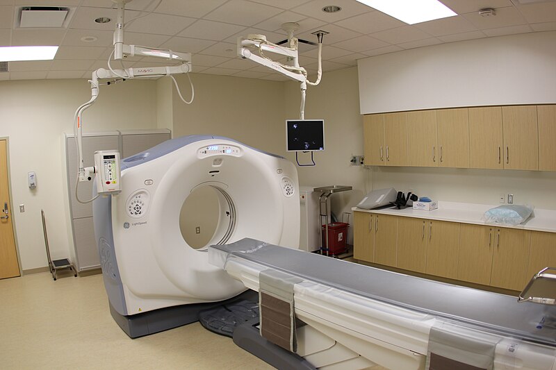
• medical: CT scan in hospitals (computed tomography)
  • 1979 Nobel price in Medicine:
    first CT scanner by Sir G.N. Hounsfield
• material science
• airport security
• accelerator physics
• ...

Projection Integral or Radon Transform $\mathcal{R}_\theta(p)$

$$\require{color} \mathcal{R}_\theta(p)\, f = \int dx\int dy~ f(x, y) \,\underbrace{\delta(x\,\cos \theta+y\,\sin\theta-p)}\limits_{\color{red}\text{projection slice}}$$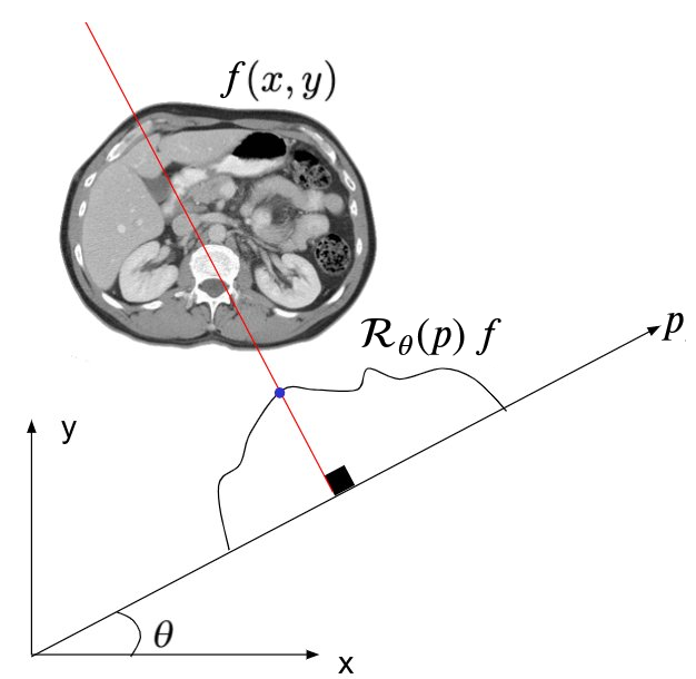

image from @docmilanfar, Twitter

Load sample image for the tomography:

data = ~np.array(Image.open('src/temf.png').convert('1', dither=False))

plt.imshow(data, cmap='binary');

Compute the Radon transform at an angle of 0 deg and 90 deg:

Rf_0 = radon(data, [0], circle=False).astype(float)
Rf_90 = radon(data, [90], circle=False).astype(float)

plt.plot(Rf_0, label='0 deg')
plt.plot(Rf_90, label='90 deg')
plt.legend()
plt.xlabel('$p$')
plt.ylabel(r'$\mathcal{R}_{\theta}(p)f$');

Preparing the Measurement Data

We take a number of VIEW measurements across the angular interval of [0,ANG] degrees:

# parameters
M = max(data.shape)
ANG = 180
VIEW = 180
THETA = np.linspace(0, ANG, VIEW, endpoint=False)

A is the projection operator, applying the Radon transform along all chosen angles THETA to the original object under study, $x$ (data):

A = lambda x: radon(x, THETA, circle=False).astype(float)

proj = A(data)

Sinogram

The sinogram represents the measurement, the collection of all projection results:

plt.imshow(proj.T)

plt.gca().set_aspect('auto')
plt.xlabel('Projection location [px]')
plt.ylabel('Rotation angle [deg]')
plt.colorbar(label='Intensity');

Reconstruction Principle

images from CERN tomography website

projection (measurement) $\implies$ back projection (reconstruction)

(Require $ N_{meas} \gtrsim \pi\cdot\frac{\text{total diameter}}{\text{pixel size}}$)

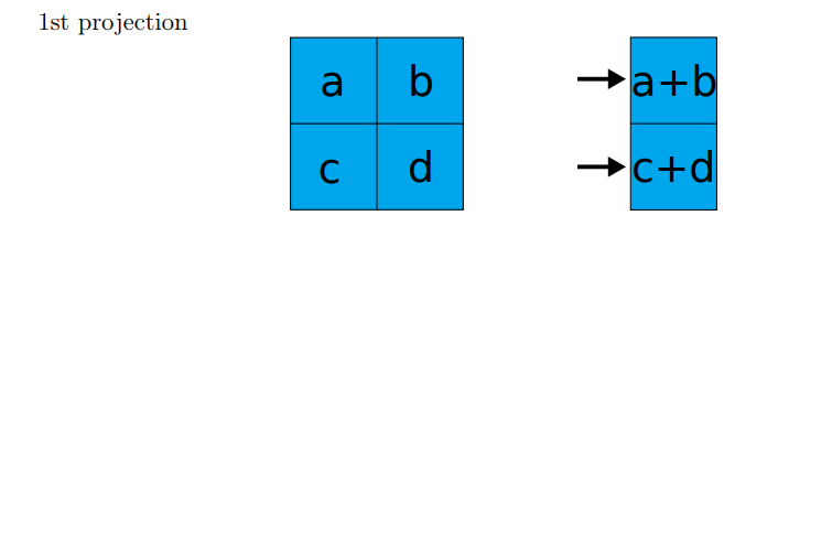
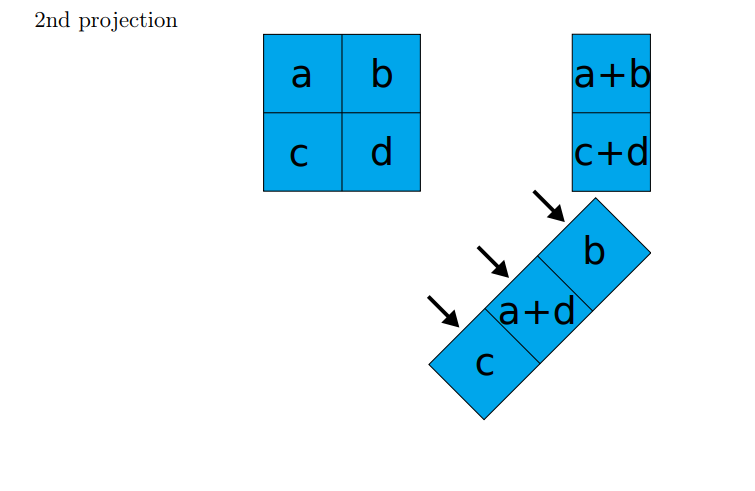
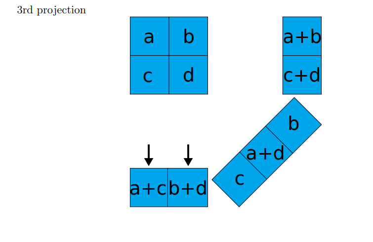
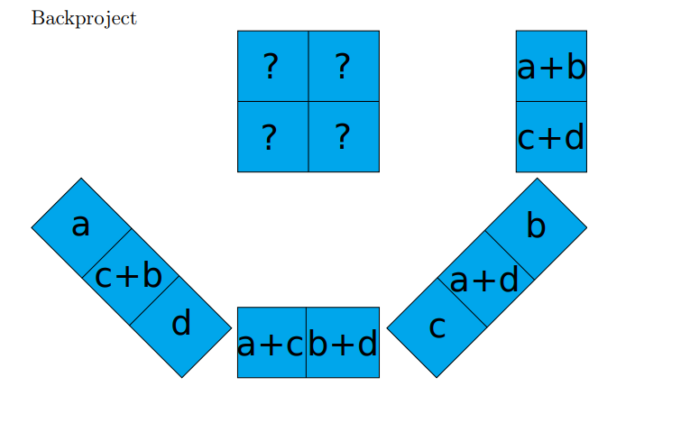
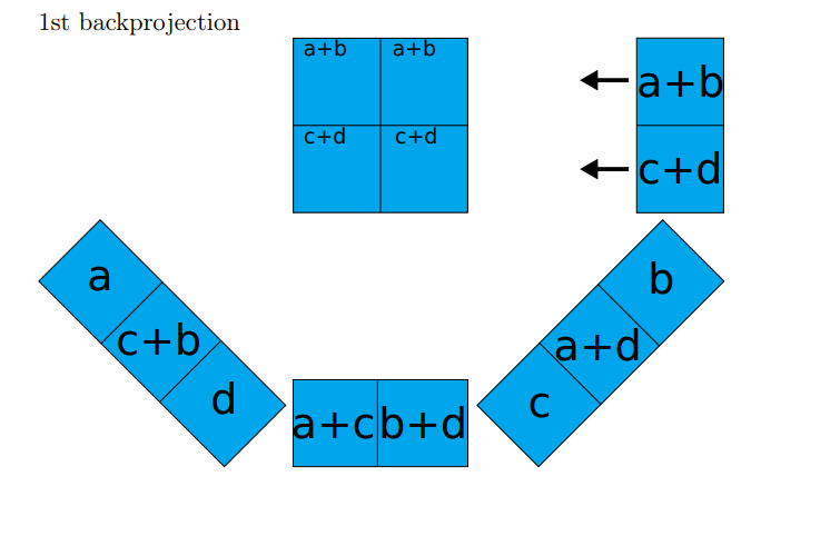
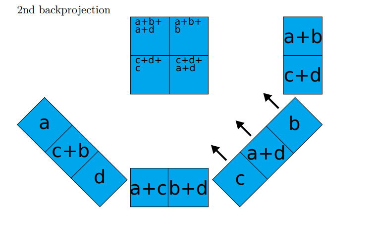
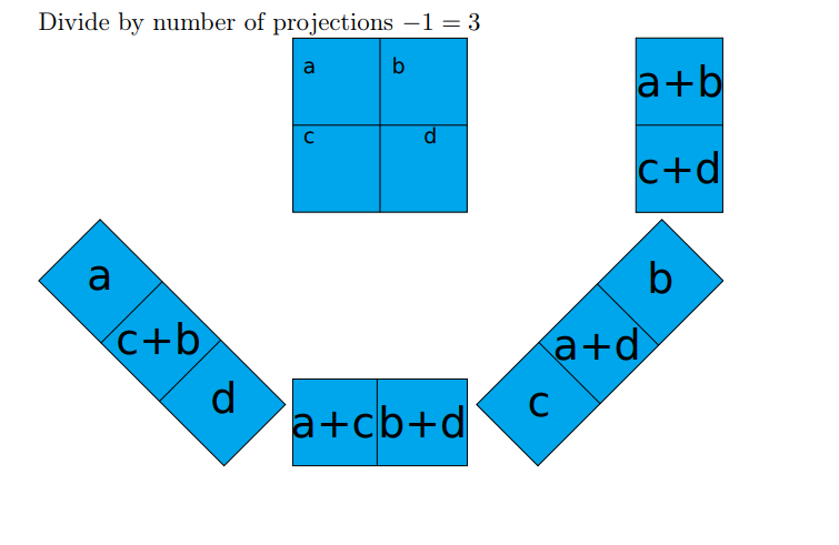
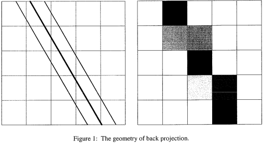
Back Projection

Information is lost where along projection line $p$ the contributions of the integral came from.

$\implies$ simple approach for the back projection:

1. simply place constant integral value along $p$ for a given angle $\theta$.
2. integrate (sum up) for all $\theta$

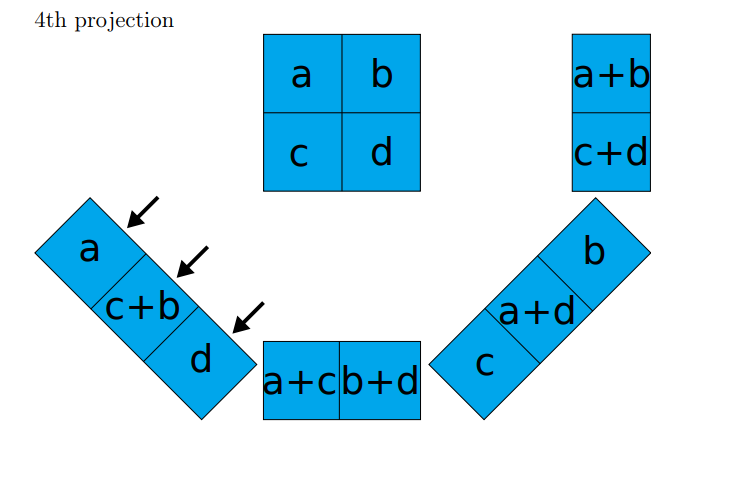
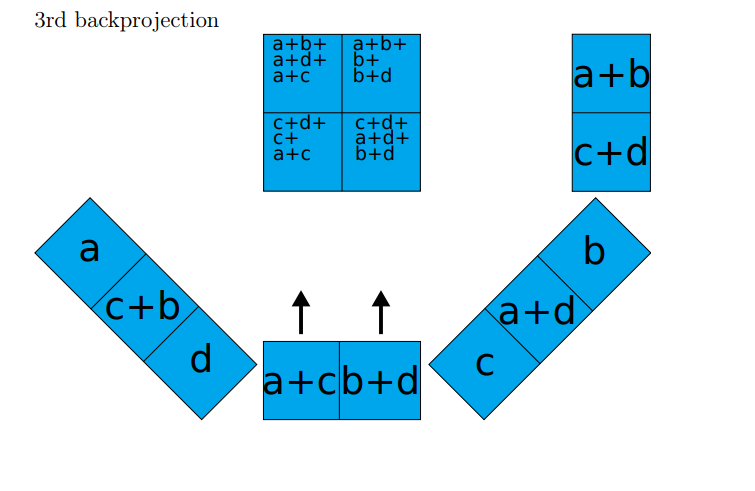
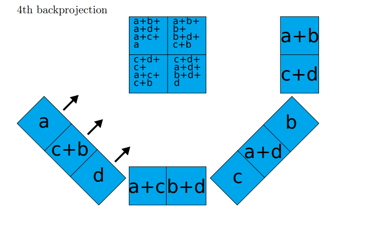
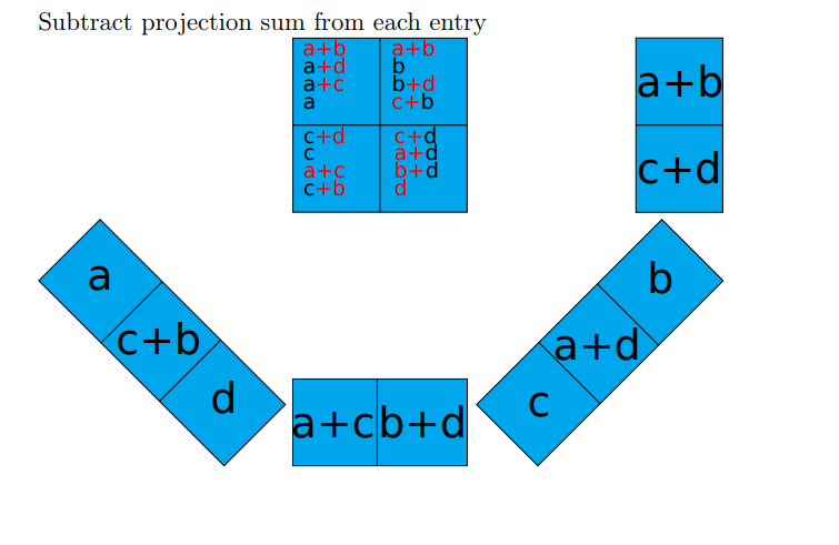
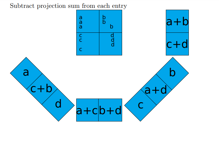
Simple Example for Back Projection

images from E. Garutti

Fourier Slice Theorem

Fourier Slice Theorem ("Projection-Slice Theorem" or "Central Slice Theorem"):

$$\mathcal{F}_\mathrm{1d}\bigl\{\mathcal{R}_{\theta'}(s) f\bigr\}=\mathcal{F}_\mathrm{2d}\bigl\{f(x,y)\bigr\}|_{\theta\mathop{=}\theta'}$$

i.e. the following two operations are equivalent:

1. project a 2D function $f(x,y)$ onto a line, 1D Fourier transform the result
2. 2D Fourier transform $f(x,y)$, extract a slice through the origin parallel to projection line

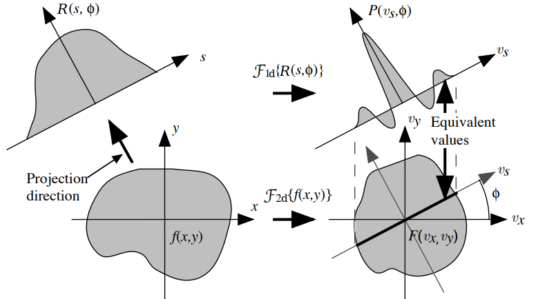
image from E. Garutti

Back Projection with FFT

Measured sinogram can be reconstructed via

1. 1D FFT of each row (projection)
2. sum up around $\theta$, interpolation in 2D Fourier space
3. inverse 2D FFT

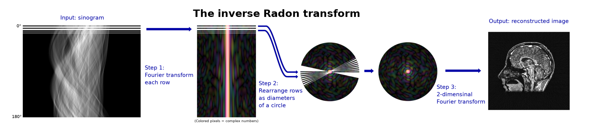
image from P. Selinger

Blurring & Filtering

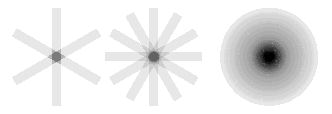
image from R. Badawi

Unfortunately, back projection oversamples the origin in Fourier space $\leadsto$ high density at low frequencies!

The "tomographic reconstruction problem": effective blurring of reconstructed image, $f(x,y)\rightarrow f(x,y)* \frac{1}{\sqrt{x^2+y^2}}$

$\implies$ solution: "ramp" filter $F(v_x,v_y)\rightarrow \sqrt{v_x^2 + v_y^2}\cdot F(v_x,v_y)$

(the price to pay: amplification of high-frequency noise components)

Using Filtered Back Projection

Let's apply the back projection as an inverse Radon transform (implemented with a ramp filter):

AINV = lambda b: iradon(b, THETA, circle=False, filter_name='ramp', output_size=M).astype(float)

fbp = AINV(proj)

plt.figure(figsize=(12, 6))
plt.imshow(fbp, cmap='binary', vmin=0, vmax=1);

$\implies$ note the artifacts due to edges in the reconstructed image (high frequency!).

Improved Reconstruction Principle

images from CERN tomography website

projection (measurement) $\implies$ back projection (reconstruction)

$\stackrel{\textcolor{red}{\text{improve}}}{\implies}$ re-projection (red) $\implies$ iteratively reduce discrepancy

Reconstruction Algorithms

image from Biomed. NMR Forschungs GmbH

image from S. Hancock

Filtered Back Projection (FBP) vs. Iterative Reconstruction

Iterative algebraic reconstruction technique (ART):
formulate reconstruction as algebraic problem $A\cdot x = b$

$\implies$ ART reconstructs $x$ iteratively
(due to sparsity of $A$, sensitivity to perturbations / noise,
direction inversion $x=A^{-1}b$ is not a useful approach!)

First suggested in 1970 by R. Gordon, R. Bender, and G. Herman for tomography!

Comparison

Filtered Back Projection	Algebraic Reconstruction Technique
FFT is fast	computationally expensive
low memory requirements	many coefficients, high memory requirements
requires many projections	more accurate, less artifacts
filtering is hard-coded into approach	can choose filtering
a-priori knowledge not possible	about distribution: straight-forward

Algebraic Reconstruction Technique

Describe the 2D density distribution under study by discrete bins (pixels), stacked into a column vector $x$.

A single projection by a ray at a given angle through the distribution is described by a row vector $a_i$. Applied to $x$, this single projection projection operation yields a pixel in a row of the sinogram, $b_i$.

The entire sinogram is collected by many projections $a_i$, which compose the (huge and sparse!) projection matrix $A_{ij}$:

$$ \sum\limits_j A_{ij} x_j = b_i $$

(each entry $x_j$ represents a discrete pixel of $x$, each $b_i$ represents a pixel in a row of the sinogram.)

Then, the algebraic reconstruction technique consists of the following iterative approximation scheme as a solution to the linear system of equations:

$$ x^{k+1} = x^k + \mu_k\frac{b_i - a_i\cdot x^k}{|a_i|^2} a_i^T $$

It converges better by introducing the (non-linear) constraint that all $x_j$ be positive, i.e. any pixel in $x$ should be set to zero if it turns negative after an iteration.

The relaxation factor $0<\mu_k\leq 1$ slows down convergence but improves the signal-to-noise ratio ($\mu_k=1$ $\rightarrow$ projection).

Effect of Noise

In the following, we will compare the FBP with the iterative ART approach on a noisy sinogram.

We add $15\%$ of the maximum sinogram value as Gaussian normal distributed noise:

noise = np.random.normal(0, 0.15 * np.max(proj), size=proj.shape)

proj_noise = proj + noise

plt.imshow(proj_noise.T)
plt.gca().set_aspect('auto')
plt.xlabel('Projection location [px]')
plt.ylabel('Rotation angle [deg]')
plt.colorbar(label='Intensity');

Filtered Back Projection Results

fbp_noise = AINV(proj_noise)

plt.imshow(fbp_noise, cmap='binary', vmin=0, vmax=1, interpolation='None');

Implement the Algebraic Reconstruction Technique

Besides the projection operator $A$, A, we need the adjoint $A^\mathrm{T}$, AT, for the ART implementation:

AT = lambda b: iradon(b, THETA, circle=False, filter_name=None, 
                      output_size=M).astype(float) * 2 * len(THETA) / np.pi

def ART(A, AT, b, x, mu=1, niter=10):
    # for all i: ||a_i||^2 = A^T ⋅ A
    ATA = AT(A(np.ones_like(x)))

    for i in tnrange(niter):
        x = x + np.divide(mu * AT(b - A(x)), ATA)

        # nonlinearity: constrain to >= 0 values
        x[x < 0] = 0

        plt.imshow(x, cmap='binary', vmin=0, vmax=1, interpolation='None')
        plt.title("%d / %d" % (i + 1, niter))
        plt.show()

    return x

# initialisation
x0 = np.zeros((M, M))
mu = 1
niter = 30

ART Results

x_art = ART(A, AT, proj_noise, x0, mu, niter)

  0%|          | 0/30 [00:00<?, ?it/s]

Comparison of the Results

ART typically outperforms FBP in terms of reconstruction quality:

_, ax = plt.subplots(1, 2, figsize=(10, 5))
plt.subplots_adjust(wspace=0.3)

plt.sca(ax[0])
plt.imshow(fbp_noise, cmap='binary', vmin=0, vmax=1, interpolation='None')
plt.title('FBP')

plt.sca(ax[1])
plt.imshow(x_art, cmap='binary', vmin=0, vmax=1, interpolation='None')
plt.title('ART');

$\implies$ the ART implementation is closely related to the Kaczmarz algorithm from numerical linear algebra.

$\implies$ Can you run tomographic reconstruction for each of the following measured sinograms?

proj = np.load('data/sinogram1.npy')
proj = np.load('data/sinogram2.npy')

Part II: Phase-space Tomography

The Concept

• tomographically reconstruct longitudinal phase-space distribution!
• sinogram: consecutive measurements of bunch profiles over many turns
• problem: non-linear motion in longitudinal phase space

$\implies$ can modify ART: construct projection matrix $A$ from tracking! Then apply usual iterative mapping!

Introduced at CERN in 1997 $\nearrow$ by Steven Hancock.

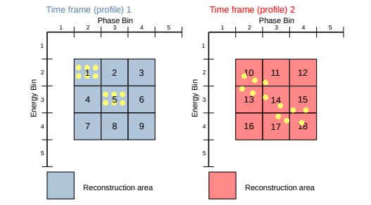
image from C. Grindheim & S. Albright

The longitudinal_tomography package is developed at CERN: control room apps tomographically reconstruct the longitudinal phase-space distribution from bunch profile measurements!

import longitudinal_tomography.tomography.tomography as tmo
from longitudinal_tomography.tracking import particles, machine

import longitudinal_tomography.utils.tomo_input as tomoin
import longitudinal_tomography.utils.tomo_output as tomoout
from longitudinal_tomography.tracking import tracking

We work once more with the PyHEADTAIL library to generate the longitudinal macro-particle distribution.

Should it not be installed yet, please run this:

!pip install PyHEADTAIL==1.16.1

Requirement already satisfied: PyHEADTAIL==1.16.1 in /home/oeftiger/anaconda3/envs/nmap23/lib/python3.10/site-packages (1.16.1)

from PyHEADTAIL.particles.generators import RFBucketMatcher, ThermalDistribution
from PyHEADTAIL.trackers.rf_bucket import RFBucket

PyHEADTAIL v1.16.1

Wall Current Monitor

In the vacuum tube, the Beam traverses a tube gap with resistors, the induced mirror current builds up voltage:

$$ V_{gap} = R_{gap} \cdot I_{beam}$$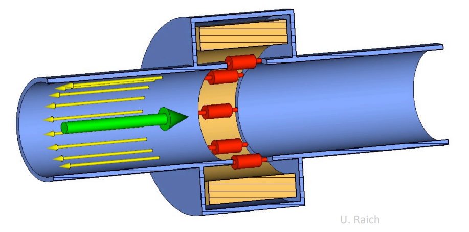

image from USPAS09 (W. Blokland, U. Raich)

Beam Measurements

Consider a circulating bunch in a synchrotron or storage ring. Longitudinal bunch profiles can be recorded via wall current monitor with a high-bandwidth oscilloscope: store $V_{gap}(t)$ during the bunch passage time $t$.

Physical beam parameters

During previous lectures we discussed reduced models for the longitudinal plane. We have

• voltage: rf voltage
• harmonic: rf frequency divided by revolution frequency
• circumference: accelerator ring circumference
• gamma: Lorentz gamma of bunch
• alpha_c: momentum compaction of the ring

voltage = 24e3
harmonic = 7
circumference = 100 * 2 * np.pi

gamma = 3.1
beta = np.sqrt(1 - gamma**-2)

alpha_c = 0.027
eta = alpha_c - gamma**-2

We look at a circulating proton bunch in a CERN Proton Synchrotron like machine. A "full bunch length" of $B_L=180\,$ns translates to an rms bunch length in meters of $\sigma_z=B_L/4 \cdot \beta c$. As before, the following PyHEADTAIL RFBucket class captures most of the important quantities for computation.

rfb = RFBucket(circumference, gamma, m_p, e, [alpha_c], 0., [harmonic], [voltage], [np.pi])

sigma_z = 180e-9 * beta * c / 4. # in [m]

A. The simulated measurement

Initialisation of particles

A thermal distribution of $N$ particles is matched into the rf bucket.

N = 100000

np.random.seed(12345)

rfb_matcher = RFBucketMatcher(rfb, ThermalDistribution, sigma_z=sigma_z)
rfb_matcher.integrationmethod = 'cumtrapz'

z, dp, _, _ = rfb_matcher.generate(N)

*** Maximum RMS bunch length 14.146533693849051m.
... distance to target bunch length: -1.2642e+01
... distance to target bunch length: 9.8693e-01
... distance to target bunch length: 9.2123e-01
... distance to target bunch length: -6.1412e-01
... distance to target bunch length: 4.1253e-01
... distance to target bunch length: 1.2473e-01
... distance to target bunch length: -1.1252e-02
... distance to target bunch length: 8.1693e-04
... distance to target bunch length: 4.9433e-06
... distance to target bunch length: -1.0032e-05
--> Bunch length: 12.769481601844392
--> Emittance: 1.8021366059891775

The distribution in longitudinal phase space $(z, \delta)$ looks as follows:

plot_mp(z, dp, rfb);

Let's have a look at the bunch profile as it would appear in a discrete measurement (e.g. via a wall current monitor):

nbins = 100
z_bins = np.linspace(*rfb.interval, num=nbins-1)

plt.hist(z, bins=z_bins, histtype='stepfilled')
plt.xlabel('$z$ [m]')
plt.ylabel('Discrete bunch profile');

A single bin of the profile measurement amounts to a time (in seconds) of

dtbin = (z_bins[1] - z_bins[0]) / (beta * c)
dtbin

3.259992054798442e-09

The synchrotron period T_s, i.e. the time period of the longitudinal motion, amounts to the following number of turns:

T_s = int(1 / rfb.Q_s)
T_s

1124

Deliberate mismatch

To provide some interesting dynamics for the tomographic reconstruction, let's mismatch the distribution in momentum. This will launch a quadrupolar oscillation, i.e. the bunch length and momentum spread will oscillate during the synchrotron period.

dp *= 0.3

As one can see, the distribution does not follow the iso-Hamiltonian lines (red) any longer but is slightly compressed along the momentum $\delta$ axis:

plot_mp(z, dp, rfb);

Particle Tracking

We model the synchrotron motion of the particles due to the rf cavities once more via a $2^\text{nd}$ order leap-frog integrator. The track function advances the particles by one turn:

def track(z, dp, rfb=rfb):
    # half drift
    z = z - eta * dp * circumference / 2
    # rf kick
    amplitude = rfb.charge * voltage / (beta * c * rfb.p0)
    phi = harmonic * (2 * np.pi * z / circumference) + rfb.phi_offset_list[0]
    dp += amplitude * np.sin(phi)
    # half drift
    z = z - eta * dp * circumference / 2
    return z, dp

Let's gather the data for the tomographic reconstruction by recording a bunch profile every few turns during one T_s:

record_every_nturns = 10

raw_data = [np.histogram(z, bins=z_bins)[0]]

for i in tnrange(1, T_s + 1):
    z, dp = track(z, dp)
    if not i % record_every_nturns:
        # the discrete WCM measurement:
        raw_data += [np.histogram(z, bins=z_bins)[0]]

  0%|          | 0/1124 [00:00<?, ?it/s]

The quadrupole oscillation is clearly visible:

plt.imshow(raw_data)
plt.xlabel('Profile bin')
plt.ylabel('#Profile')
plt.colorbar(label='Density');

$\implies$ Can you explain when the shortest bunch length (the bright spot with peak density) occurs? Why does one expect the shortest bunch length here, given the initial condition of the mismatched momentum distribution (with factor 0.3)?

plt.plot(np.std(raw_data, axis=1))
plt.xlabel('#profile')
plt.ylabel('rms buhch length [arb.units]');

$\implies$ a $\gtrsim 100\%$ rms bunch length (quadrupole) oscillation takes place!

Ready...

We have now gathered a simulated discrete WCM measurement in the raw_data array during one synchrotron period.

B. The longitudinal tomographic reconstruction

Preparations

The longitudinal_tomography package requires a certain input format for the machine parameters (voltage, frequency, etc):

frame_input_args = {
    'raw_data_path':    './',
    'framecount':       len(raw_data), # Number of frames in input data
    'skip_frames':      0, # Number of frames to ignore
    'framelength':      len(raw_data[0]), # Number of bins in each frame
    'dtbin':            dtbin, # Width (in s) of each frame bin
    'skip_bins_start':  0, # Number of frame bins before the lower profile bound to ignore
    'skip_bins_end':    0, # Number of frame bins after the upper profile bound to ignore
    'rebin':            1, #Number of frame bins to rebin into one profile bin
}

# computation of dipole B-field from beam rigidity Brho = p/e
Ekin = (gamma - 1) * m_p * c**2 / e
p0c = np.sqrt(Ekin**2 + 2*Ekin*m_p/e * c**2)
brho = p0c / c
brho / 70.08

0.13104352797152807

machine_args = {
    'output_dir':           '/tmp/', # Directory in which to write all output
    'dtbin':                dtbin, # Width (in s) of each frame bin
    'dturns':               record_every_nturns, # Number of machine turns between frames
    'synch_part_x':         frame_input_args['framelength']/2, # Time (in frame bins) 
                            # from the lower profile bound to the synchronous phase (if <0, 
                            # a fit is performed) in the "bunch reference" frame
    'demax':                -1e6, # noqa - Max energy (in eV) of reconstructed phase space (if >0)
    'filmstart':            0, # Number of the first profile at which to reconstruct
    'filmstop':             1, # Number of the last profile at which to reconstruct
    'filmstep':             1, # Step between reconstructions
    'niter':                50, # Number of iterations for each reconstruction
    'snpt':                 4, # Square root of the number of test particles to track per cell
    'full_pp_flag':         False, # Flag to extend the region in phase space of map elements (if =1)
    'beam_ref_frame':       0, # Reference frame for bunch parameters (synchronous phase, baseline, integral)
    'machine_ref_frame':    0, # Reference frame for machine parameters (RF voltages, B-field)
    'vrf1':                 voltage, # Peak RF voltage (in V) of principal RF system
    'vrf1dot':              0.0, # and its time derivative (in V/s)
    'vrf2':                 0.0, # Peak RF voltage (in V) of higher-harmonic RF system
    'vrf2dot':              0.0, # and its time derivative (in V/s)
    'h_num':                harmonic, # Harmonic number of principal RF system
    'h_ratio':              2.0, # Ratio of harmonics between RF systems
    'phi12':                0, # Phase difference (in radians of the principal harmonic) between RF systems
    'b0':                   brho / 70.08, # Dipole magnetic field (in T) -- up to 1.8T
    'bdot':                 0.0, # and its time derivative (in T/s) -- up to 10T/s
    'mean_orbit_rad':       circumference / (2 * np.pi), # Machine radius (in m)
    'bending_rad':          70.08, # Bending radius (in m)
    'trans_gamma':          alpha_c**-0.5, # Gamma transition
    'rest_energy':          m_p * c**2 / e, # Rest mass (in eV/c**2) of accelerated particle
    'charge':               1, # Charge state of accelerated particle
    'self_field_flag':      False, # Flag to include self-fields in the tracking (if =1)
    'g_coupling':           0.0, # Geometrical coupling coefficient
    'zwall_over_n':         0.0, # Reactive impedance (in Ohms per mode number) over a machine turn
    'pickup_sensitivity':   1, # Effective pick-up sensitivity (in digitizer units per instantaneous Amp)
    'nprofiles':            frame_input_args['framecount'],
    'nbins':                frame_input_args['framelength'],
    'min_dt':               0.0,
    'max_dt':               dtbin * frame_input_args['framelength'],
}

# initialising tomography
frames = tomoin.Frames(**frame_input_args)

mach = machine.Machine(**machine_args)

mach.values_at_turns()

The tomography package uses the waterfall plot of profiles as measured sinogram input then:

measured_waterfall = frames.to_waterfall(np.array(raw_data, dtype=float).flatten())

plt.imshow(measured_waterfall)
plt.xlabel('Profile bin')
plt.ylabel('#Profile')
plt.colorbar(label='Density');

Settings

Reconstruction will be carried out at the following profile index:

(choose 0 for the first profile, or -2 for the last, or any number < len(measured_waterfall) - 1)

reconstr_idx = 0

Number of iterations of ART:

niterations = 50

Projection Matrix

Establishing the map via tracking (nonlinear synchrotron motion), i.e. matrix $A$:

tracker = tracking.Tracking(mach)

phip, dEp = tracker.track(reconstr_idx)

# Converting from physical coordinates ([rad], [eV])
# to internal phase space coordinates.
if not tracker.self_field_flag:
    phip, dEp = particles.physical_to_coords(
        phip, dEp, mach, tracker.particles.xorigin,
        tracker.particles.dEbin)

phip, dEp = particles.ready_for_tomography(phip, dEp, mach.nbins)

profiles = tomoin.raw_data_to_profiles(
    measured_waterfall, mach, frames.rebin, frames.sampling_time)
profiles.calc_profilecharge()

waterfall = profiles.waterfall

# further preparations
nprofs = waterfall.shape[0]
nbins = waterfall.shape[1]
nparts = phip.shape[0]

flat_profs = waterfall.copy()
flat_profs = flat_profs.clip(0.0)

flat_profs /= np.sum(flat_profs, axis=1)[:, None]
flat_profs = np.ascontiguousarray(flat_profs.flatten()).astype(float)

waterfall /= np.sum(waterfall, axis=1)[:, None]

flat_points = phip.copy()
for i in range(nprofs):
    flat_points[:, i] += nbins * i

Starting the algebraic reconstruction technique (ART) algorithm:

# Initialising arrays with zeros
weight = np.zeros(nparts)
rec_wf = np.zeros(waterfall.shape)

# Initial estimation of weight factors using (flattened) measured profiles.
weight = tmo.libtomo.back_project(weight, flat_points, flat_profs,
                                  nparts, nprofs)
weight = weight.clip(0.0)

diff = []
for i in range(niterations):
    # Projection from phase space to time projections
    rec_wf = tmo.libtomo.project(rec_wf, flat_points, weight, nparts,
                                 nprofs, nbins)

    # Normalizing reconstructed waterfall
    rec_wf /= np.sum(rec_wf, axis=1)[:, None]

    # Finding difference between measured and reconstructed waterfall
    dwaterfall = waterfall - rec_wf

    # Setting to zero for next round
    rec_wf[:] = 0.0

    # Calculating discrepancy
    diff.append(np.sqrt(np.sum(dwaterfall**2) / (nbins * nprofs)))

    # Back projection using the difference between measured and recorded waterfall
    weight = tmo.libtomo.back_project(weight, flat_points, dwaterfall.flatten(),
                                      nparts, nprofs)
    # non-linearity of ART:
    weight = weight.clip(0.0)

    print(f'Iteration: {i:3d}, discrepancy: {diff[-1]:3e}')

Iteration:   0, discrepancy: 9.043262e-03
Iteration:   1, discrepancy: 7.403652e-03
Iteration:   2, discrepancy: 6.275827e-03
Iteration:   3, discrepancy: 5.433833e-03
Iteration:   4, discrepancy: 4.773068e-03
Iteration:   5, discrepancy: 4.241804e-03
Iteration:   6, discrepancy: 3.804729e-03
Iteration:   7, discrepancy: 3.437714e-03
Iteration:   8, discrepancy: 3.124893e-03
Iteration:   9, discrepancy: 2.854680e-03
Iteration:  10, discrepancy: 2.618902e-03
Iteration:  11, discrepancy: 2.411621e-03
Iteration:  12, discrepancy: 2.228095e-03
Iteration:  13, discrepancy: 2.064704e-03
Iteration:  14, discrepancy: 1.918603e-03
Iteration:  15, discrepancy: 1.787428e-03
Iteration:  16, discrepancy: 1.669183e-03
Iteration:  17, discrepancy: 1.562216e-03
Iteration:  18, discrepancy: 1.465202e-03
Iteration:  19, discrepancy: 1.377001e-03
Iteration:  20, discrepancy: 1.296639e-03
Iteration:  21, discrepancy: 1.223286e-03
Iteration:  22, discrepancy: 1.156163e-03
Iteration:  23, discrepancy: 1.094654e-03
Iteration:  24, discrepancy: 1.038225e-03
Iteration:  25, discrepancy: 9.863460e-04
Iteration:  26, discrepancy: 9.385863e-04
Iteration:  27, discrepancy: 8.945884e-04
Iteration:  28, discrepancy: 8.539385e-04
Iteration:  29, discrepancy: 8.163688e-04
Iteration:  30, discrepancy: 7.815886e-04
Iteration:  31, discrepancy: 7.493189e-04
Iteration:  32, discrepancy: 7.193588e-04
Iteration:  33, discrepancy: 6.915095e-04
Iteration:  34, discrepancy: 6.656000e-04
Iteration:  35, discrepancy: 6.414583e-04
Iteration:  36, discrepancy: 6.189430e-04
Iteration:  37, discrepancy: 5.979151e-04
Iteration:  38, discrepancy: 5.782955e-04
Iteration:  39, discrepancy: 5.599825e-04
Iteration:  40, discrepancy: 5.428430e-04
Iteration:  41, discrepancy: 5.267852e-04
Iteration:  42, discrepancy: 5.117289e-04
Iteration:  43, discrepancy: 4.975914e-04
Iteration:  44, discrepancy: 4.843117e-04
Iteration:  45, discrepancy: 4.718202e-04
Iteration:  46, discrepancy: 4.600484e-04
Iteration:  47, discrepancy: 4.489418e-04
Iteration:  48, discrepancy: 4.384692e-04
Iteration:  49, discrepancy: 4.285785e-04

# Finding last discrepancy...
rec_wf = tmo.libtomo.project(rec_wf, flat_points, weight, nparts, nprofs, nbins)
rec_wf /= np.sum(rec_wf, axis=1)[:, None]
dwaterfall = waterfall - rec_wf
diff.append(np.sqrt(np.sum(dwaterfall**2) / (nbins * nprofs)))

print(f'Iteration: {i + 1:3d}, discrepancy: {diff[-1]:3E}')

Iteration:  50, discrepancy: 4.192405E-04

Reconstruction finished, return the reconstructed phase-space distribution:

phasespace = tomoout.create_phase_space_image(
    phip, dEp, weight, nbins, reconstr_idx)

Results from Tomography

The profile of the reconstructed distribution compared to the input profile:

prof_rec = np.sum(phasespace, axis=1)
z_rec = (0.5 + np.arange(-len(prof_rec)/2, len(prof_rec)/2)) * (-dtbin * beta * c)

plt.plot(z_rec, prof_rec, label='reconstructed')
plt.plot(z_rec, waterfall[reconstr_idx], label='measured')

plt.xlabel('$z$ [m]')
plt.ylabel('Histogram')
plt.legend(loc='upper left', bbox_to_anchor=(1.05, 1));

The reconstructed rms bunch length is: $\sigma_z = \sqrt{\cfrac{\sum_i p(z_i) \cdot (z_i - \langle z \rangle)^2}{\sum_i p(z_i)}}$

np.sqrt(np.trapz(prof_rec * z_rec**2, z_rec) / np.trapz(prof_rec, z_rec))

12.78047289439187

The original macro-particle distribution was generated with:

sigma_z

12.769476658495181

The momentum distribution of the reconstructed distribution:

Etot = Ekin + m_p/e * c**2 # in eV

profdp_rec = np.sum(phasespace, axis=0)
dp_rec = (0.5 + np.arange(-len(profdp_rec)/2, len(profdp_rec)/2)) * (tracker.particles.dEbin / (Etot) * beta**2)

plt.plot(dp_rec, profdp_rec)
plt.xlabel('$\delta$')
plt.ylabel('Reconstructed histogram');

The reconstructed rms momentum deviation is: $\sigma_\delta = \sqrt{\cfrac{\sum_i p(\delta_i) \cdot (\delta_i - \langle \delta \rangle)^2}{\sum_i p(\delta_i)}}$

np.sqrt(np.trapz(profdp_rec * dp_rec**2, dp_rec) / np.trapz(profdp_rec, dp_rec))

0.0003310112038759302

Here is the full reconstructed phase-space distribution:

plot_tomo(phasespace, z_rec, dp_rec, rfb);

Does this fit the initial macro-particle distribution? (Scroll up to section A. to compare!)

Mind that this tomogram is reconstructed purely from the spatial projections (the simulated WCM measurements), the tomography algorithm has no knowledge of the macro-particles and their phase-space distribution!!

$\implies$ Re-run the tomographic reconstruction for the last profile (see settings part above, start from section B.)! Does it match the final macro-particle distribution?

The final macro-particle phase-space distribution after the simulation:

plot_mp(z, dp, rfb);

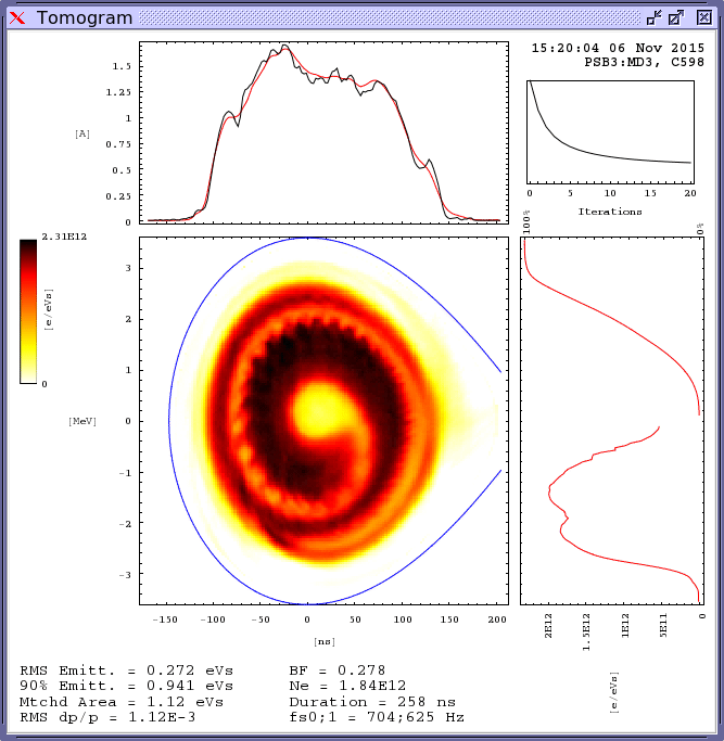
$\implies$ Reconstruct some tomograms from actual measurements in the CERN PS Booster:

1. phase space filamentation
2. "string of pearls": digital rf phase feedback too strong

The last example is also found on the CERN tomography website $\nearrow$, where you find further nice tomography applications.

Summary

• Radon transform for line projections, construction of sinogram
• Reconstruction of $n$-dimensional distributions from $(n-1)$-dimensional projections
• Fourier Slice Theorem
• Filtered Back Projection
• Algebraic Reconstruction Technique
• Phase-space Tomography (concept: construction of projection matrix $A$ via non-linear tracking)

Original material used for this lecture

• Y. Han's github repository on ART

A nice dedicated lecture on Iterative Algorithms:

• Lecture on Algebraic Methods for Computed Tomography at TU of Denmark