Numerical Methods in Accelerator Physics
Lecture Series by Dr. Adrian Oeftiger

Lecture 2
Run this notebook online!
Interact and run this jupyter notebook online:
Also find this lecture rendered as HTML slides on github $\nearrow$ along with the source repository $\nearrow$.
Run this first!
Imports and modules:
from config import (np, plt, hamiltonian,
                    plot_hamiltonian, solve_leapfrog,
                    get_boundary_ids, set_axes,
                    plot_macro_evolution, dt)
%matplotlib inline
Refresher!
- accelerators $=$ $1 + \epsilon$ $=$ single-particle dynamics + perturbative multi-particle dynamics
- bending and focusing concept
- linacs vs. cyclotrons vs. synchrotrons
- synchrotron time scales: transverse oscillations vs. longitudinal oscillations vs. storage time
- phase space
- equations of motion and the Hamiltonian
- discrete integration
- Liouville theorem, symplecticity
Today!
- RMS Emittance and Preservation
- Discrete Frequency Analysis
Coordinate System in Accelerators
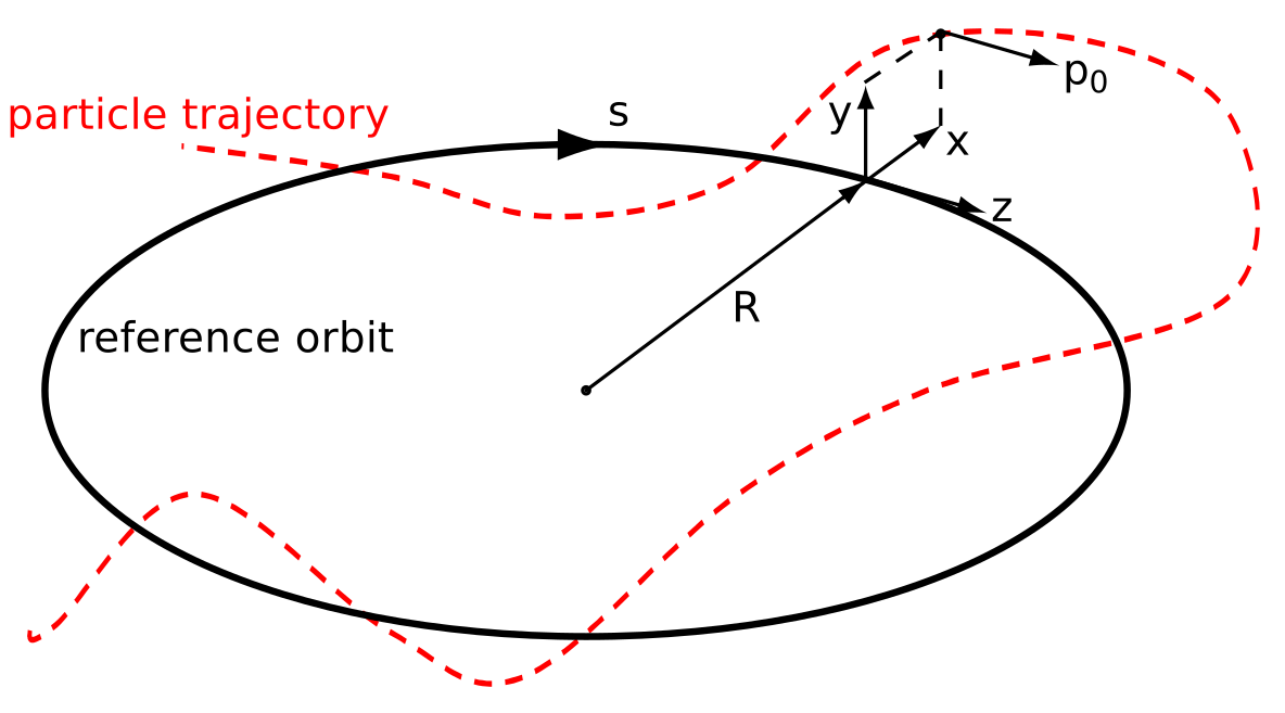
Reference orbit: ideal trajectory through magnets in accelerator
Path length $s$: independent time-like parameter following reference particle with momentum $p_0=\beta\gamma m_0 c$ in longitudinal direction
Particle 3D position in accelerator is measured as 3D offset from the reference orbit position at path length $s$:
$$(x,y,z)$$$$\begin{align} x& \text{: horizontal offset [m]} \\ y& \text{: vertical offset [m]} \\ z& \text{: longitudinal offset [m]} \end{align}$$Conjugate Momenta
Longitudinal momentum in the direction of motion $p_z$.
Transverse momenta $P_x, P_y$ are typically expressed as trajectory slopes: $$\begin{align}\, x' &\doteq \frac{dx}{ds} = \frac{P_x}{p_z} \\ y' &\doteq \frac{dy}{ds} = \frac{P_y}{p_z} \end{align}$$
$\leadsto$ Paraxial approximation: $x'\ll 1,~ y'\ll 1,~ p_z\approx p_0$
$\implies$ measure $p_z$ as momentum offset from $p_0$: $\delta = \frac{p_z - p_0}{p_0}$
6D Phase Space
A point particle $\implies$ occupies a point in 6D phase space:
$$\zeta = \begin{pmatrix} x \\ x' \\ y \\ y' \\ z \\ \delta \end{pmatrix}$$In typical synchrotron situations: horizontal $(x,x')$ and vertical $(y,y')$ phase space are decoupled!
$\implies$ will study when this approximation applies during derivation of reduced transverse and longitudinal models!
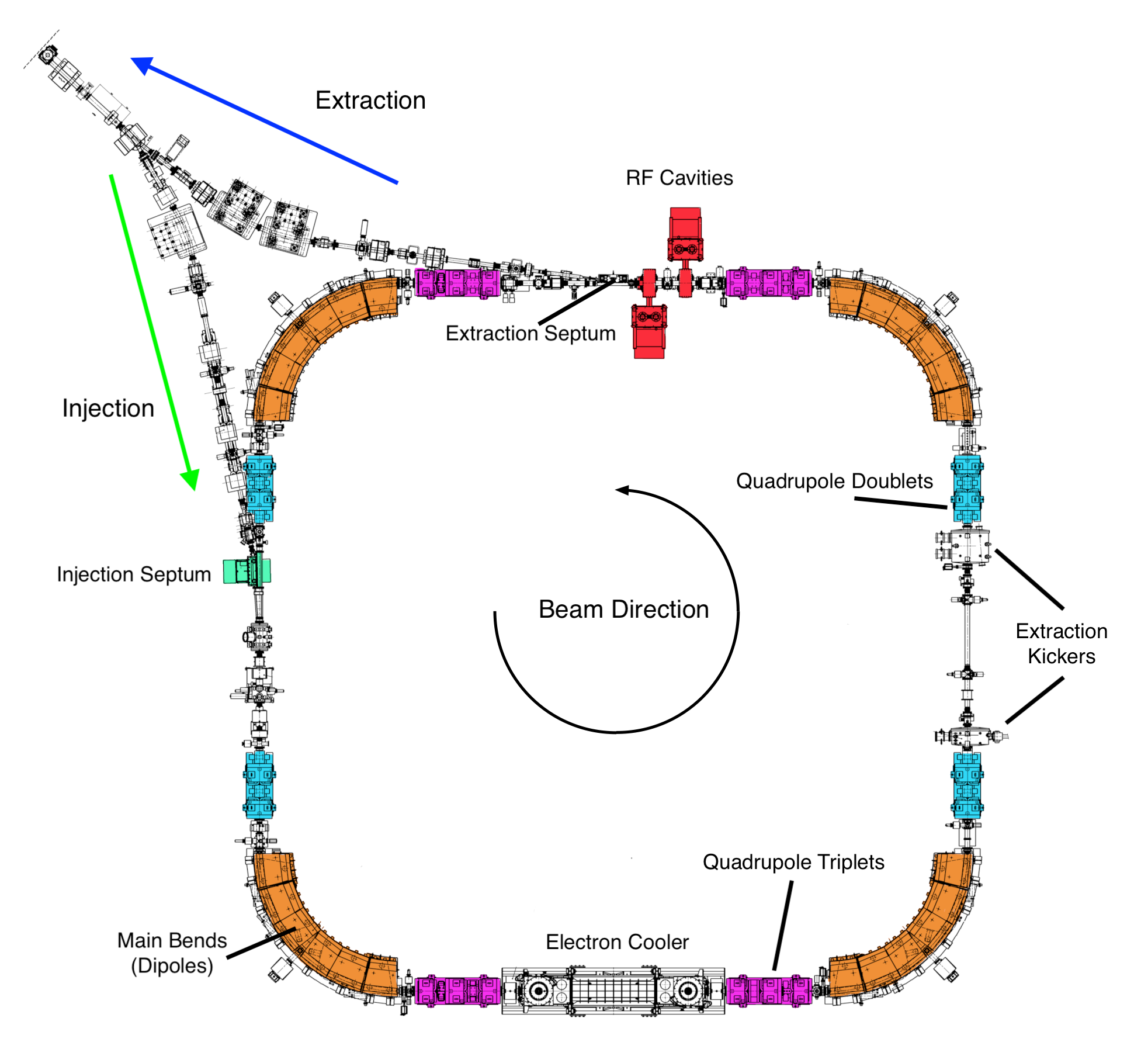
Analogy of Pendulum with Accelerator
Longitudinal phase focusing with rf cavities:
- particles drift over most of the circular accelerator
- particles get kicked only in rf cavities
(energy change through standing electromagnetic wave)
$\implies$ closely corresponds to discrete pendulum situation!
Let's simulate collection of pendulums
Create distribution of initial conditions $(\theta_i, p_i)$ for the pendulum (like a beam of $N$ particles):
theta_grid = np.linspace(-0.5 * np.pi, 0.5 * np.pi, 21)
p_grid = np.linspace(-0.3, 0.3, 5)

thetas, ps = np.meshgrid(theta_grid, p_grid)
N = len(theta_grid) * len(p_grid)
N
105
plt.scatter(thetas, ps, c='b', marker='.')

plot_hamiltonian()

$\implies$ rectangular distribution (reminds of a beam pulse injected from a linac)
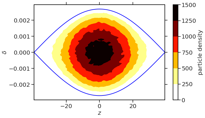
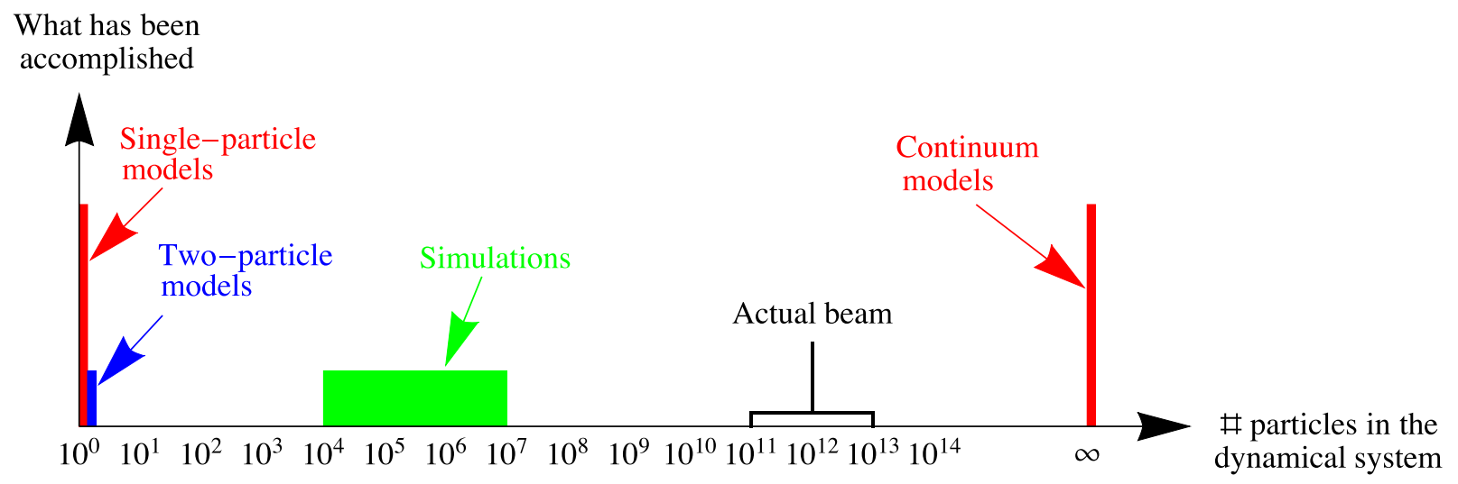
Beam Emittance
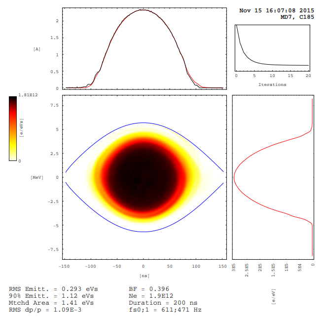
Beam distribution: $10^{11}...10^{13}$ particles
$\epsilon=$ rms of all particle amplitudes!
Moment of a distribution
Measure statistical moments of a distribution of $N$ particles/states in phase space:
$$\langle f(\zeta) \rangle \doteq \frac{1}{N}\sum\limits_i^N f(\zeta_i)$$where $f$ is a monomial of the phase-space coordinates, e.g.
$$\begin{cases} \langle x \rangle: & \text{horizontal centroid (centre-of-mass)} \\ \sigma_y = \sqrt{\left\langle \bigl(y - \langle y \rangle \bigr)^2\right\rangle} = \sqrt{\langle y^2 \rangle - \langle y\rangle^2}: & \text{vertical rms beam size} \end{cases}$$$\implies$ what is the order of the monomial moments $\langle x\rangle$ and $\sigma_y$?
Statistical RMS Emittance
Measure extent of distribution in phase space via $\Sigma$-matrix, the covariance matrix of second-order moments, e.g. for horizontal phase space (assume for simplicity $\langle x\rangle=\langle x'\rangle=0$):
$$\Sigma_x = \begin{pmatrix} \langle x^2\rangle & \langle x\,x'\rangle \\ \langle x\,x'\rangle & \langle x'{}^2\rangle \\ \end{pmatrix}$$$\implies$ the rms emittance is given by:
$\leadsto$ a value for the "thermal energy" of the distribution
(for $\langle x\rangle,\langle x'\rangle\neq 0$ need to subtract them: $x\mapsto x-\langle x\rangle$ and $x'\mapsto x'-\langle x'\rangle$)
Time evolution
Numerical integration of equations of motion for distribution of pendulums, using leapfrog (drift+kick+drift):
n_steps = 100
results_thetas = np.zeros((n_steps, N), dtype=np.float32)
results_thetas[0] = thetas.flatten()

results_ps = np.zeros((n_steps, N), dtype=np.float32)
results_ps[0] = ps.flatten()

for k in range(1, n_steps):
    results_thetas[k], results_ps[k] = solve_leapfrog(results_thetas[k - 1], results_ps[k - 1])
Observations of Centroids
Before we look at all "particles" (pendulums), check evolution of some distribution moments:
centroids_theta = 1/N * np.sum(results_thetas, axis=1)
centroids_p = 1/N * np.sum(results_ps, axis=1)
plt.plot(centroids_theta, label=r'$\langle\theta\rangle$')
plt.plot(centroids_p, label=r'$\langle p\rangle$')

plt.xlabel('Steps $k$')
plt.ylabel('Centroid amplitude')
plt.legend(bbox_to_anchor=(1.05, 1));

$\implies$ can you explain this?
Observations of RMS Sizes
Before we look at all "particles" (pendulums), check evolution of some distribution moments:
var_theta = 1/N * np.sum(results_thetas * results_thetas, axis=1)
var_p = 1/N * np.sum(results_ps * results_ps, axis=1)
plt.plot(var_theta, label=r'$\langle\theta^2\rangle$')
plt.plot(var_p, label=r'$\langle p^2\rangle$')

plt.xlabel('Steps $k$')
plt.ylabel('Variance')
plt.legend(bbox_to_anchor=(1.05, 1));

$\implies$ can you explain this?
Mismatch of Distributions
Non-linearity of the pendulum equation: decreased oscillation frequency at larger amplitudes!
A) matched distribution:
B) mismatched distribution:
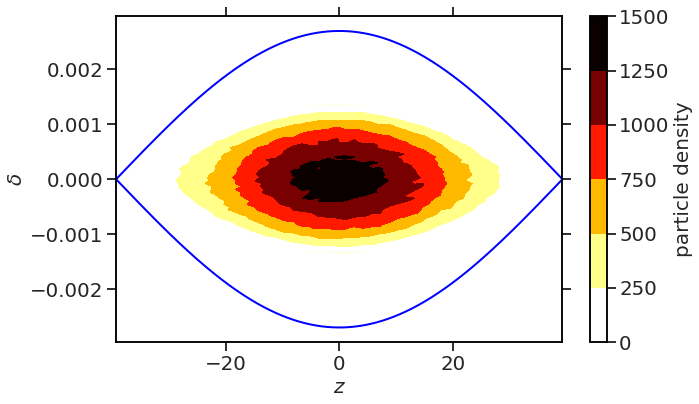
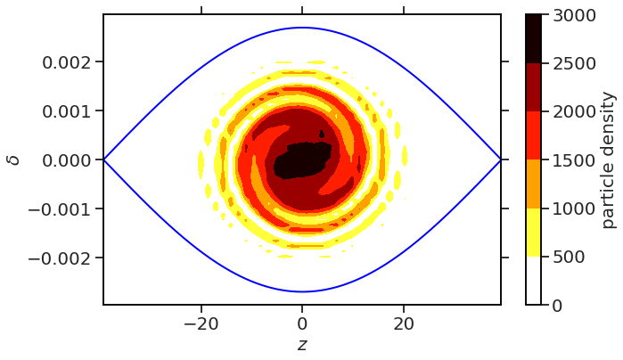
Filamentation
- Liouville theorem (incompressible phase-space fluid) still valid, local density conserved
- occupied global phase-space area by beam seemingly enlarged
- reason: filamentation due to non-linearity:
$\implies$ non-linear potential $\longrightarrow$ oscillation frequency depends on amplitude $\implies$ anharmonicity - consequence: rms emittance increases (in previous example: $\Delta\epsilon/\epsilon=30\%$)
Back to our pendulum simulation:
Observe distribution evolution over the $k$ steps:
k = 0

plt.scatter(results_thetas[k], results_ps[k], c='b', marker='.')

plot_hamiltonian()
RMS Emittance Evolution
Let us compute the rms emittance for the pendulums (having subtracted the centroids),
$$\epsilon = \sqrt{\langle \theta^2\rangle \langle p^2\rangle - \langle \theta\,p\rangle^2}$$def emittance(theta, p):
N = len(theta)
# subtract centroids
theta = theta - 1/N * np.sum(theta)
p = p - 1/N * np.sum(p)
# compute Σ matrix entries
theta_sq = 1/N * np.sum(theta * theta)
p_sq = 1/N * np.sum(p * p)
crossterm = 1/N * np.sum(theta * p)
# determinant of Σ matrix
epsilon = np.sqrt(theta_sq * p_sq - crossterm * crossterm)
return epsilon
results_emit = np.zeros(n_steps, dtype=np.float32)

for k in range(n_steps):
    results_emit[k] = emittance(results_thetas[k], results_ps[k])
plt.plot(results_emit)

plt.xlabel('Steps $k$')
plt.ylabel('RMS emittance $\epsilon$');

$\implies$ rms emittance grows, macroscopic increase of "thermal energy"!
Microscopic Level?
What about Liouville theorem?
$\implies$ For the symplectic integrator, we still expect (and have) constant phase-space trajectory density!
$\implies$ what happens when one integrates around a very small area and follows it during the simulation?
Emittance vs. Linear Dynamics
$\implies$ What happens with the rms emittance in case of linear dynamics (absence of non-linearities)?
Exercise:
- Taylor-expand the sine function in the pendulum equations of motion
- cut after first order: $\sin\theta \approx \theta + \mathcal{O}(\theta^3)$
- re-run the simulation for this linear system (why is this system linear now?)
- observe the variances as well as emittance evolution!
- can you explain why the emittance behaves this way (in contrast to non-linear model?)
Hint: the definition of the leapfrog integrator function needs to be changed for your simulation in this exercise:
def solve_leapfrog(theta, p, dt=dt):
    theta_half = theta + dt / 2 * p / (m * L*L)
    p_next = p - dt * m * g * L * np.sin(theta_half)
    theta_next = theta_half + dt / 2 * p_next / (m * L*L)
    return (theta_next, p_next)
Note: Modelling error
Typical example:
$\implies$ Taylor-expand potential $U\propto \sin\theta$ to a certain finite order
$\implies$ large amplitudes are behaved differently from original pendulum!
$\implies$ error in approximation $=$ modelling error
(in contrast to discretisation error, see last lecture)
Centroid offset in (Original) Pendulum
Consider again the non-linear pendulum: let us offset the initial centroid $\langle \theta\rangle$!
results_thetas2 = np.zeros((n_steps, N), dtype=np.float32)
results_thetas2[0] = thetas.flatten() + 0.1 * np.pi

results_ps2 = np.zeros((n_steps, N), dtype=np.float32)
results_ps2[0] = ps.flatten()

for k in range(1, n_steps):
    results_thetas2[k], results_ps2[k] = solve_leapfrog(results_thetas2[k - 1], results_ps2[k - 1])
$\implies$ will the rms emittance growth be smaller / equal / larger?
Observation of Centroids II
centroids_theta2 = 1/N * np.sum(results_thetas2, axis=1)
centroids_p2 = 1/N * np.sum(results_ps2, axis=1)

plt.plot(centroids_theta, label=r'no offset: $\langle\theta\rangle$')
plt.plot(centroids_theta2, label=r'with offset: $\langle\theta\rangle$')
plt.plot(centroids_p2, label=r'with offset: $\langle p\rangle$')

plt.xlabel('Steps $k$')
plt.ylabel('Centroid amplitude')
plt.legend(bbox_to_anchor=(1.05, 1));

RMS Emittance Evolution II
results_emit2 = np.zeros(n_steps, dtype=np.float32)

for k in range(n_steps):
    results_emit2[k] = emittance(results_thetas2[k], results_ps2[k])
plt.plot(results_emit, label='no offset')
plt.plot(results_emit2, label='with offset')

plt.xlabel('Steps $k$')
plt.ylabel('RMS emittance $\epsilon$')
plt.legend();

Long-term Behaviour
n_steps = 3000
results_thetas3 = np.zeros((n_steps, N), dtype=np.float32)
results_thetas3[0] = thetas.flatten() + 0.1 * np.pi

results_ps3 = np.zeros((n_steps, N), dtype=np.float32)
results_ps3[0] = ps.flatten()

for k in range(1, n_steps):
    results_thetas3[k], results_ps3[k] = solve_leapfrog(results_thetas3[k - 1], results_ps3[k - 1])
plot_macro_evolution(results_thetas3, results_ps3);

$\implies$ Observations:
- oscillations of all moments dampen out until residual noise level
- emittance growth saturates rather quickly
Important Notes on RMS Emittance Evolution
Reminder of Basic Thermodynamic Principle: $\delta S \geq 0$
RMS emittance:
- constant or grows for conservative forces (closed systems)
- in accelerator systems, only ways to reduce / dampen emittance:
- synchrotron radiation
- electron cooling
- stochastic cooling (Nobel prize: van de Meer)
Emittance Preservation
$\implies$ avoid injection mismatch when transferring
beam between accelerators:
- centroid mismatch
- rms beam size mismatch
$\implies$ avoid resonances / instabilities
$\implies$ require accurate numerical simulation models for predictions!
Summing Up Concepts
- non-linearities in dynamical system $\implies$ oscillation frequency depends on amplitude $\implies$ anharmonicity
- microscopic: Liouville (density of phase-space trajectories conserved)
- macroscopic: filamentation
- rms emittance: macroscopic extent of distribution in phase space
- control of simulation errors: discretisation errors, modelling errors, numerical artefacts (see later!)
Continuous Pendulum: Linear Oscillation Frequency
Reminder:
Equation of motion: $$\frac{d^2\theta}{dt^2} + \frac{g}{L}\sin\theta = 0$$
for $\sin\theta\approx \theta$: $$\implies \frac{d^2\theta}{dt^2} + \underbrace{\frac{g}{L}}\limits_{\mathop{=}\omega^2}\theta = 0$$
During a time step $\Delta t=0.1$, the phase advance (in units of 2π) gives:
freq_theory = np.sqrt(1 / 1) * 0.1 / (2 * np.pi)
freq_theory
0.015915494309189534
Determining Oscillation Frequencies
Can we quantify the change of oscillation frequency towards larger amplitudes?
$\implies$ DFT: Discrete Fourier Transform technique
$$f_n = \sum\limits_{k=0}^{N_\mathrm{step}-1} \theta_{k}\,e^{-i2\pi\frac{n}{N_\mathrm{step}} k}$$Obtain frequency components $f_n$ from signal $\theta_k$ recorded over $N_\mathrm{step}$ steps.
FFT: Efficient Algorithm for $N_{step}=2^\ell$
Fast Fourier Transform (FFT): among 10 most influential algorithms in 20th century!
- continuous splitting of DFT summation:
- exploiting symmetry identify of DFT: $f_{n+jN_\mathrm{step}} = f_{n}$ for $j=0,1,2...$
- basic DFT: complexity $\mathcal{O}(N_\mathrm{step}^2)$
- vs. FFT: complexity $\mathcal{O}(N_\mathrm{step}\,\log_2 N_\mathrm{step})$
$\implies$ can you compare the time required for DFT vs. FFT for $N_\mathrm{step}=10^9$ and 1 ns time per compute operation?
Employ FFT on Pendulum Motion
Observe two particles:
i1 = N // 2 - 10
i2 = N // 2

plt.plot(results_thetas3[:, i1])
plt.plot(results_thetas3[:, i2])
plt.xlabel('Steps $k$')
plt.ylabel(r'$\theta$');

Obtain the FFT spectra for both:
spec1 = np.fft.rfft(results_thetas3[:, i1])
spec2 = np.fft.rfft(results_thetas3[:, i2])

freq = np.fft.rfftfreq(n_steps)
plt.plot(freq, np.abs(spec1))
plt.plot(freq, np.abs(spec2))
plt.axvline(freq_theory, c='k', zorder=0, ls='--')
plt.xlim(0, 0.05)
plt.xlabel('Phase advance per $\Delta t$ [$2\pi$]')
plt.ylabel('FFT spectrum')
plt.yscale('log');

Frequency vs. Amplitude
Let us plot the maximum frequency vs. initial $\theta$ (where $p=0$):
specs = np.abs(np.fft.rfft(results_thetas3.T))
max_ids = np.argmax(specs, axis=1)
amplitudes = np.max(specs, axis=1)
i_range = np.where(ps.flatten() == 0)[0]

plt.scatter(results_thetas3[0][i_range], freq[max_ids][i_range])

plt.axhline(freq_theory, c='k', ls='--', zorder=0)
plt.xticks([-np.pi/2, 0, np.pi/2, np.pi], [r"$-\pi/2$", "0", r"$\pi/2$", r"$\pi$"])
plt.xlabel(r'Initial $\theta$ ($p=0$)')
plt.ylabel('Phase advance / \n' + r'integration step $\Delta t$ [$2\pi$]');
plt.ylim(0.012, 0.0165);

$\implies$ what is responsible for the step behaviour / finite resolution of the vertical values? How would you further increase the resolution in this plot?
The NAFF Algorithm
J. Laskar describes in 1989: "The Chaotic Motion of the Solar System: A Numerical Estimate of the Size of Chaotic Zones"
NAFF $=$ Numerical Analysis of Fundamental Frequencies
$\implies$ quasi-periodic decomposition: iterative fitting of (not necessarily orthogonal) fundamental frequencies for numerical signal over finite time span.
In accelerator physics, sometimes find equivalent formulation as SUSSIX algorithm.
Usage:
- celestial mechanics
- particle accelerators
- atomic physics
- general dynamical system issues (Hamiltonian dynamics, chaos)
Frequency Accuracy for Periodic Motion
FFT: maximum distance to the nearest FFT resolved frequency is $\frac{1}{2N_\mathrm{step}\Delta t}$, i.e. the frequency accuracy scales with
$$\Delta f_\mathrm{FFT} \propto \frac{1}{\Delta t}$$NAFF: based on the Hanning window implementation, the frequency accuracy scales with
$$\Delta f_\mathrm{NAFF} \propto \frac{1}{\color{red}{\Delta t^4}}$$import PyNAFF
freqs_naff = []

for signal in results_thetas3.T[i_range]:
    freq_naff = PyNAFF.naff(signal, turns=n_steps - 1, nterms=1)
    try:
        freq_naff = freq_naff[0, 1]
    except IndexError:
        freq_naff = 0
    freqs_naff += [freq_naff]

freqs_naff = np.array(freqs_naff)
plt.scatter(results_thetas3[0][i_range], freq[max_ids][i_range])
plt.plot(results_thetas3[0][i_range], freqs_naff, c='r', marker='.')

plt.axhline(freq_theory, c='k', ls='--', zorder=0)
plt.xticks([-np.pi/2, 0, np.pi/2, np.pi], [r"$-\pi/2$", "0", r"$\pi/2$", r"$\pi$"])
plt.xlabel(r'Initial $\theta$ ($p=0$)')
plt.ylabel('Phase advance / \n' + r'integration step $\Delta t$ [$2\pi$]');

plt.plot(results_thetas3[0][i_range], 100 * (freq[max_ids][i_range] - freqs_naff) / freqs_naff)
plt.xlabel(r'Initial $\theta$ ($p=0$)')
plt.ylabel('Error (FFT - NAFF) / NAFF ' + r'[%]');

Summary
- statistical moments
- rms emittance
- filamentation: microscopic level Liouville vs. macroscopic emittance growth
- emittance preservation and injection mismatch
- modelling error (in addition to discretisation error last lecture)
- discrete frequency analysis: FFT and NAFF