Numerical Methods in Accelerator Physics
Lecture Series by Dr. Adrian Oeftiger

Lecture 1
Run this notebook online!
Interact and run this jupyter notebook online:
Also find this lecture rendered as HTML slides on github $\nearrow$ along with the source repository $\nearrow$.
Run this first!
Imports and modules:
from config import *
%matplotlib inline
Today!
- About Accelerators
- Time Scales
- Modelling a Pendulum ($\leadsto$ rf cavities focusing a beam)
Accelerator Physics
Accelerator physics $\Longleftrightarrow$ plasma physics
- single-particle effects: non-linear dynamics
- multi-particle effects: collective instabilities
What is an "accelerator"?
$$\begin{array}\,\text{beam self fields} &>& \text{external applied fields} &\text{(plasma)} \\ \text{beam self fields} &\ll& \text{external applied fields}& \text{(accelerator)}\end{array}$$$\implies$ perturbation technique applicable to higher-energy accelerators:
$$\begin{cases} \text{unperturbed motion} &=& \text{external fields} \\ \text{perturbation} &=& \text{self fields} \end{cases}$$Large part of this course: model effects on particle beam due to external fields!
Accelerator Fundamentals
Putting it simple: 3 major ingredients
- radio frequency (rf) cavities for bunching and acceleration
- dipole magnets for steering
- quadrupole magnets for (transverse) focusing
$\implies$ enforce oscillations to contain particles!
One "Electron Volt"
1 eV $=$ gained kinetic energy of particle with elementary charge after traversing 1 V potential difference
Common Higher-energy Accelerator Types
Cyclotrons
- low energy (limited by relativistic effects)
- protons/ions
- provide muons, neutrons, isotopes
- medical applications and research
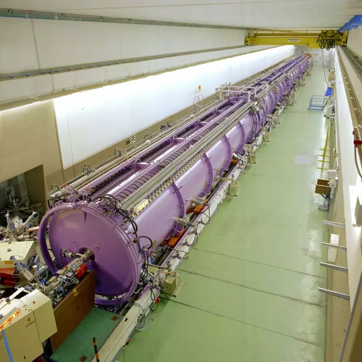
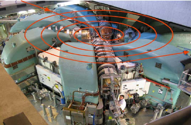 image: PSI cyclotron, Villigen (CH)
Synchrotrons
- highest energies
- slowly ramp up energy of beam
- protons/ions: fundamental research
- electrons: synchrotron light sources
 image: LEIR at CERN, Geneva (CH)
FAIR complex at GSI
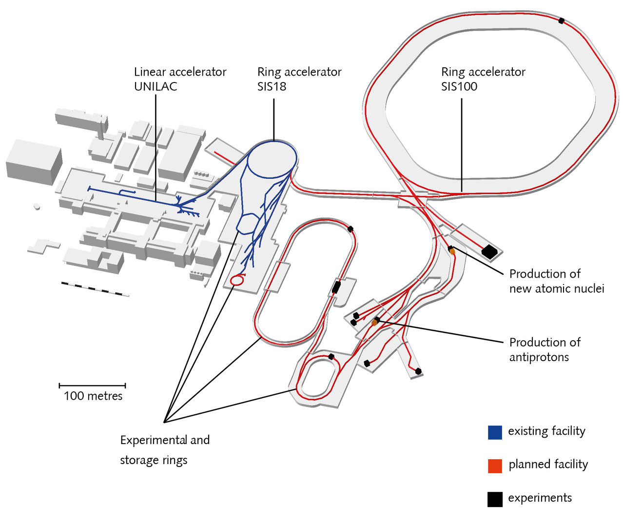
Protons..Uranium for FAIR experiments:
- UNILAC: $\sim$ 11 MeV/u
- SIS18: $\leq$ 1 GeV/u (Uranium) or 4.5 GeV (protons)
- SIS100: $\leq$ 10 GeV/u (Uranium) or 29 GeV (protons)
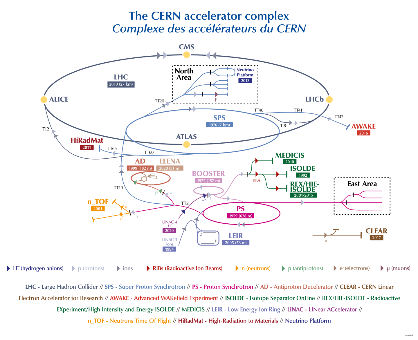
CERN complex
Protons for LHC injection:
- LINAC4: 160 MeV
- PSB: 2 GeV
- PS: 26 GeV
- SPS: 450 GeV
- LHC: 7 TeV
World-record LHC Fill Duration
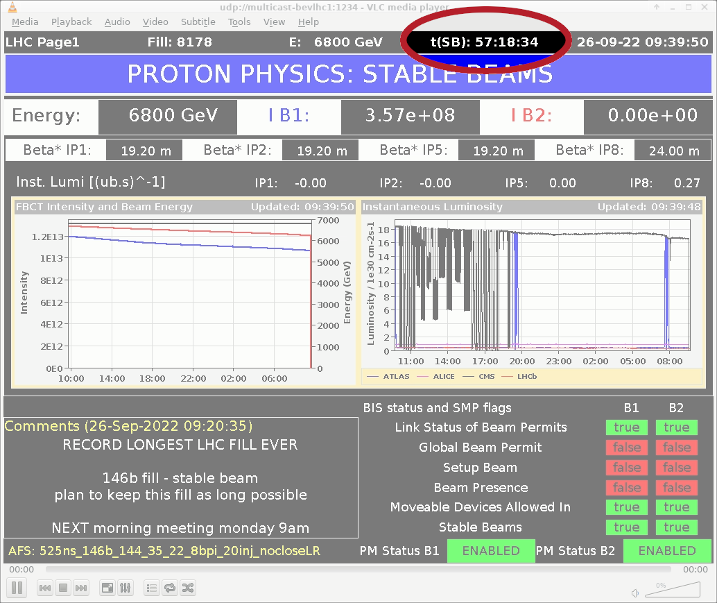
image: CERN LHC OP logbook 2022
$\leadsto$ 57h of beam storage $=$ how many turns in 27 km long LHC?
Time Scales in a Synchrotron
A turn $\sim$ 1..100 μs:
- many per turn: transverse (betatron) oscillations
- once per turn: observation in a wall current monitor
- 100s of turns: longitudinal (synchrotron) oscillations
- 100s of turns: $e$-fold damping time of feedback systems
- 100'000s to $>$ millions of turns: storage times
(compare: stability of the Earth's orbit around the Sun (age: 4.6 My))
Accuracy Required!
Analytical models do not suffice for quantitative understanding!
$\implies$ require detailed numerical models
$\implies$ predict and control stability over these time scales!
$\implies$ learn about basic concepts in this lecture! :-)
In the following...
Use simple pendulum to demonstrate development of numerical simulation model!
Clarify concepts:
- phase space, Hamiltonian
- discrete integration
- symplecticity
- 3 error sources of such simulation models:
- discretisation
- next time: numerical artefacts, modelling errors
The Nonlinear Pendulum
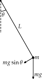
- point mass $m$ suspended on (weightless/inextensible) rod of length $L$
- gravitational acceleration $g$ pulls $m$ downwards
- degree of freedom: displacement angle $\theta$ of $m$ over time $t$
$\implies$ second-order non-linear ODE (ordinary differential equation)
$\leadsto$ numerical integration should give expected periodic movement!
Phase Space
Very useful concept in classical mechanics:
- collect all states of dynamical system
- for $i$ degrees of freedom:
each coordinate $q_i$ has associated conjugate momentum $p_i$ - momentary state vector $(q_i, p_i)$ evolves with time $t$
- equations of motion (e.o.m.) connect $(q_i, p_i)$ with each other:
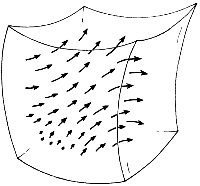
phase-space trajectories are solution of e.o.m. - rich structure, "symplectic manifold", phase space $=$ incompressible fluid:
- phase-space trajectories are unique $\implies$ never overlap/cross
- Liouville's theorem: local trajectory density does not change
image: Roger Penrose,
The Road of Reality
$\implies$ we will clarify via examples!
Conjugate Momentum
Consider $$p \doteq m L^2 \frac{d\theta}{dt}$$
(use Lagrangian functional to construct $p$ -- not focus of this lecture, see e.g. here for more details)
2nd-order ODE equation of motion $\leadsto$ 2 coupled 1st-order ODEs: evolution of $(\theta, p)$
$$\frac{d^2\theta}{dt^2} + \frac{g}{L}\sin\theta = 0 \quad \Longleftrightarrow \quad \left\{\begin{array}\, \cfrac{d\theta}{dt} &= \cfrac{p}{mL^2} \\ \cfrac{dp}{dt} &= -m g L\sin\theta \end{array}\right.$$Let's plot in phase space!
m = 1
g = 1
L = 1
def plot_arrow(theta, p, dt=1):
    # equations of motion:
    dtheta = p / (m * L*L) * dt
    dp = - m * g * L * np.sin(theta) * dt

    # plotting
    plt.scatter([theta], [p], s=50, c='r', marker='*', zorder=10)
    plt.annotate('',
                 xytext=(theta, p),
                 xy=(theta + dtheta, p + dp),
                 arrowprops=dict(facecolor='black', shrink=0.03))
plot_arrow(1, 0)
# plot_arrow(0, -1)
# plot_arrow(-1, 0)
# plot_arrow(0, 1)
# plot_arrow(1/1.41, 1/1.41)

# # increase momentum:
# for i in np.arange(0.4, 2.5, 0.2):
#     plot_arrow(0, i)

# # increase angle:
# for i in np.arange(1, np.pi * 1.1, 0.2):
#     plot_arrow(i, 0)

set_axes()

Conservation of Energy
Equation of motion for $\theta(t)$: $$\frac{d^2\theta}{dt^2} + \frac{g}{L}\sin\theta = 0$$
$$\begin{align} \text{Potential energy}:& &U &= mgL(1 - \cos\theta) \\ \text{Kinetic energy}:& &T &= \frac{1}{2}mL^2\left(\frac{d\theta}{dt}\right)^2 \end{align}$$The Hamiltonian
$\mathcal{H} \doteq T + U$ is an example of a Hamiltonian functional on $\theta(t),p(t)$.
- integral of motion (total energy) when $\mathcal{H}$ not explicitly depending on time
- equations of motion $=$ gradient of Hamiltonian w.r.t. phase-space coordinates $(q_i,p_i)$
- in 2D: contours of constant Hamiltonian value $=$ phase-space trajectories
Hamiltonian of the Pendulum
$$\mathcal{H} = T + U = \frac{1}{2} \frac{p^2}{mL^2} + m g L \left(1 - \cos\theta\right)$$and correspondingly the 2 coupled 1D equations of motion via the Hamilton equations:
$$\left.\begin{array}\, \cfrac{d\theta}{dt} = \cfrac{\partial\mathcal{H}}{\partial p} \\ \cfrac{dp}{dt} = -\cfrac{\partial\mathcal{H}}{\partial\theta} \end{array}\right\} \quad \Longleftrightarrow \quad \left\{\begin{array}\, \cfrac{d\theta}{dt} &= \cfrac{p}{mL^2} \\ \cfrac{dp}{dt} &= -m g L\sin\theta \end{array}\right.$$def hamiltonian(theta, p):
T = p * p / (2 * m * L*L)
U = m * g * L * (1 - np.cos(theta))
return T + U
TH, PP = np.meshgrid(np.linspace(-np.pi * 1.1, np.pi * 1.1, 100),
                     np.linspace(-3, 3, 100))

HH = hamiltonian(TH, PP)

plt.contour(TH, PP, HH, levels=10)
plt.colorbar(label=r'$\mathcal{H}(\theta, p)$')

set_axes()

TH, PP = np.meshgrid(np.linspace(-np.pi * 1.1, np.pi * 1.1, 100),
                     np.linspace(-3, 3, 100))

HH = hamiltonian(TH, PP)

plt.contourf(TH, PP, HH, cmap=plt.get_cmap('hot_r'))
plt.colorbar(label=r'$\mathcal{H}(\theta, p)$')

plot_arrow(2, 0)

set_axes()

Observations: Pendulum Phase-space Topology
- origin $(0,0)$: stable fixed point
- bound motion (circular phase-space trajectories) close to origin
($\Leftrightarrow$ pendulum swinging back and forth) - at larger angles towards $|\theta|\lesssim \pi$ change of angle slows down
- unstable fixed points at $|\theta|=\pi$
- unbound motion (continuous phase-space trajectories) at large momenta
($\Leftrightarrow$ pendulum moves in one angular direction only) - separatrix: phase-space boundary separating bound from unbound motion
Summing up Concepts
- phase space: all momentary states $(\theta, p)$ of the dynamical system
- Hamiltonian $\mathcal{H}$: shapes landscape / geometry of phase space $\implies$ equations of motion
$\implies$ let's go ahead and apply discrete integrators to simulate the pendulum
$\leadsto$ Hamiltonian contours indicate exact geometry of solutions to the pendulum e.o.m. for comparison
Discretisation
differential equation with continuous parameter $t$ $\stackrel{\text{discretise}}{\implies}$ discrete map with time steps $t=k\Delta t$
Start with Forward Integration
Assume constant values during $\Delta t$: "Explicit Euler method"
$$\left.\begin{array}\, \cfrac{d\theta}{dt} &= \cfrac{p}{mL^2} \\ \cfrac{dp}{dt} &= -m g L\sin\theta \end{array}\right\} \quad \stackrel{\text{Euler}}{\Longrightarrow} \quad \left\{\begin{array}\, \theta_{k+1} &= \theta_k + \Delta t\cdot\cfrac{p_{k}}{mL^2} \\ p_{k+1} &= p_k - \Delta t\cdot m g L\sin\theta_k \end{array}\right.$$def solve_euler(theta, p, dt=0.1):
theta_next = theta + dt * p / (m * L*L)
p_next = p - dt * m * g * L * np.sin(theta)
return (theta_next, p_next)
theta_ini = -1.1
p_ini = 0
n_steps = 100
results_euler = np.zeros((n_steps, 2), dtype=np.float32)
results_euler[0] = (theta_ini, p_ini)

for k in range(1, n_steps):
    results_euler[k] = solve_euler(*results_euler[k - 1])
plt.contour(TH, PP, HH, levels=10, linestyles='--', linewidths=1)

plt.plot(results_euler[:, 0], results_euler[:, 1], c='b')

set_axes()

$\implies$ Is there something qualitatively wrong with our integrator?
Total Energy should be conserved?
plt.plot(
    hamiltonian(results_euler[:, 0], results_euler[:, 1]),
    c='b', label='Euler integrator')
plt.axhline(hamiltonian(theta_ini, p_ini), c='r', label='theory')

plt.xlabel('Steps $k$')
plt.ylabel(r'$\mathcal{H}(\theta, p)$')
plt.legend();

$\implies$ discrete pendulum model violates energy conservation
Even worse:
theta_ini2 = -3.
p_ini2 = 0
n_steps = 100
results_euler2 = np.zeros((n_steps, 2), dtype=np.float32)
results_euler2[0] = (theta_ini2, p_ini2)

for k in range(1, n_steps):
    results_euler2[k] = solve_euler(*results_euler2[k - 1])
plt.contour(TH, PP, HH, levels=10, linestyles='--', linewidths=1)
plt.plot(results_euler2[:, 0], results_euler2[:, 1], c='b')
set_axes()

Change from bound to unbound region?
Hamiltonian value of separatrix: $\mathcal{H}_{sep} = \mathcal{H}(-\pi, 0)\qquad$ (at unstable fixed point)
h_sep = hamiltonian(-np.pi, 0)
h_sep
2.0
plt.plot(
    hamiltonian(results_euler2[:, 0], results_euler2[:, 1]),
    c='b', label='Euler integrator')
plt.axhline(hamiltonian(theta_ini2, p_ini2), c='r', label='theory')
plt.axhline(h_sep, c='k', label='$\mathcal{H}_{sep}$')

plt.xlabel('Steps $k$')
plt.ylabel(r'$\mathcal{H}(\theta, p)$')
plt.legend(bbox_to_anchor=(1.05, 1))
plt.ylim(top=2.1);

Conclusion from Euler Integrator
- violates energy conservation: increasing energy / amplitude continuously
- even breaks underlying structure of original phase space: leaving bound motion region to unbound region
(... think of implications for predicting LHC stability or Earth's orbit)
Symplecticity
Euler method is a non-symplectic integrator, i.e. breaks Hamiltonian nature and Liouville theorem.
Instead, numerical integrator mapping should preserve phase-space density (be symplectic)!
$\implies$ Jacobian $\mathbb{J}$ of map should satisfy $\det(\mathbb{J})\mathop{\stackrel{!}{=}} 1$
Euler method violates this, e.g. for pendulum:
$$\mathbb{J}_{Euler} = \begin{pmatrix} \cfrac{\partial\theta_{k+1}}{\partial\theta_k} & \cfrac{\partial\theta_{k+1}}{\partial p_k} \\ \cfrac{\partial p_{k+1}}{\partial\theta_k} & \cfrac{\partial p_{k+1}}{\partial p_k} \end{pmatrix} = \begin{pmatrix} 1 & \cfrac{\Delta t}{mL^2} \\ -\Delta t\, mgL\cos\theta_k & 1 \end{pmatrix} \implies \det\left(\mathbb{J}_{Euler}\right) \neq 1$$Euler-Cromer Method
Let's fix symplecticity / phase-space volume preservation!
Euler has approximation error $\mathcal{O}(\Delta t^2)$.
$\implies$ add cancellation term of same magnitude (simplify $m=L=g=1$):
$$\mathbb{J}_{EC} = \begin{pmatrix} 1 & \Delta t \\ -\Delta t\cos\theta_k & 1 \color{red}{-\Delta t^2\cos\theta_k} \end{pmatrix} $$Euler-Cromer Method II
Main difference to Euler method: "staircase" movement in phase space
- first update $\theta$
- then update $p$
Euler-Cromer Method III
Illustration of stair-case movement in phase space for linear pendulum where $\sin\theta\approx \theta$:
$$\left\{\begin{array}\, \theta_{k+1} &= \theta_k + \Delta t\cdot p_{k} \\ p_{k+1} &= p_k - \Delta t\cdot \color{red}{\theta_{k+1}} \end{array}\right. \\[2em] \stackrel{\text{Jacobian}}{\Longrightarrow} \quad \mathbb{J}_{EC} = \begin{pmatrix} 1 & \Delta t \\ -\Delta t & 1 \color{red}{-\Delta t^2} \end{pmatrix} = \underbrace{\begin{pmatrix} 1 & 0 \\ -\Delta t & 1 \end{pmatrix}}\limits_\text{"kick": update $p$} \cdot \underbrace{\begin{pmatrix} 1 & \Delta t \\ 0 & 1 \end{pmatrix}}\limits_\text{"drift": update $\theta$} $$$\implies$ Euler-Cromer method is sometimes referred to as drift-kick algorithm
Implement in Python
def solve_eulercromer(theta, p, dt=0.1):
    ### from Euler:
    theta_next = theta + dt * p / (m * L*L)
    p_next = p - dt * m * g * L * np.sin(theta_next)
    return (theta_next, p_next)
results_eulercromer = np.zeros((n_steps, 2), dtype=np.float32)
results_eulercromer[0] = (theta_ini, p_ini)

for k in range(1, n_steps):
    results_eulercromer[k] = solve_eulercromer(*results_eulercromer[k - 1])
plt.contour(TH, PP, HH, levels=10, linestyles='--', linewidths=1)

plt.plot(results_euler[:, 0], results_euler[:, 1], c='b', label='Euler')
plt.plot(results_eulercromer[:, 0], results_eulercromer[:, 1], c='c', label='Euler-Cromer')

plt.legend(bbox_to_anchor=(1.05, 1))
set_axes()

What about energy conservation now?
plt.plot(
    hamiltonian(results_euler[:, 0], results_euler[:, 1]),
    c='b', label='Euler')
plt.plot(
    hamiltonian(results_eulercromer[:, 0], results_eulercromer[:, 1]),
    c='c', label='Euler-Cromer')
plt.axhline(hamiltonian(theta_ini, p_ini), c='r', label='theory')

plt.xlabel('Steps $k$')
plt.ylabel(r'$\mathcal{H}(\theta, p)$')
plt.legend(bbox_to_anchor=(1.05, 1));

$\implies$ still finite error -- but bound within an interval around the correct solution!
(In fact, a modified Hamiltonian $\mathcal{K}$ is conserved...)
Adding Mid-point Rule: $\mathcal{O}(\Delta t^3)$
Störmer-Verlet (or "leapfrog") method: staggered update, formulate as drift-kick-drift!
 $$\left.\begin{array}\,
\cfrac{d\theta}{dt} &= \cfrac{p}{mL^2} \\
\cfrac{dp}{dt} &= -m g L\sin\theta
\end{array}\right\} \quad \stackrel{\text{leapfrog}}{\Longrightarrow} \quad \left\{\begin{array}\,
\theta_{\color{red}{k+1/2}} &= \theta_k + \color{red}{\cfrac{\Delta t}{2}}\cdot\cfrac{p_{k}}{mL^2} \\
p_{k+1} &= p_k - \Delta t\cdot m g L\sin\theta_\color{red}{{k+1/2}} \\
\theta_{\color{red}{k+1}} &= \theta_{\color{red}{k+1/2}} + \color{red}{\cfrac{\Delta t}{2}}\cdot\cfrac{p_{\color{red}{k+1}}}{mL^2}
\end{array}\right.$$
$$\left.\begin{array}\,
\cfrac{d\theta}{dt} &= \cfrac{p}{mL^2} \\
\cfrac{dp}{dt} &= -m g L\sin\theta
\end{array}\right\} \quad \stackrel{\text{leapfrog}}{\Longrightarrow} \quad \left\{\begin{array}\,
\theta_{\color{red}{k+1/2}} &= \theta_k + \color{red}{\cfrac{\Delta t}{2}}\cdot\cfrac{p_{k}}{mL^2} \\
p_{k+1} &= p_k - \Delta t\cdot m g L\sin\theta_\color{red}{{k+1/2}} \\
\theta_{\color{red}{k+1}} &= \theta_{\color{red}{k+1/2}} + \color{red}{\cfrac{\Delta t}{2}}\cdot\cfrac{p_{\color{red}{k+1}}}{mL^2}
\end{array}\right.$$Exercise: verify that Jacobian of leapfrog algorithm gives $\det\left(\mathbb{J}_\text{leapfrog}\right) = 1$
def solve_leapfrog(theta, p, dt=0.1):
    theta_half = theta + dt / 2 * p / (m * L*L)
    p_next = p - dt * m * g * L * np.sin(theta_half)
    theta_next = theta_half + dt / 2 * p_next / (m * L*L)
    return (theta_next, p_next)
results_leapfrog = np.zeros((n_steps, 2), dtype=np.float32)
results_leapfrog[0] = (theta_ini, p_ini)

for k in range(1, n_steps):
    results_leapfrog[k] = solve_leapfrog(*results_leapfrog[k - 1])
plt.plot(
    hamiltonian(results_euler[:, 0], results_euler[:, 1]),
    c='b', label='Euler, $\mathcal{O}(\Delta t^2)$')
plt.plot(
    hamiltonian(results_eulercromer[:, 0], results_eulercromer[:, 1]),
    c='c', label='Euler-Cromer, $\mathcal{O}(\Delta t^2)$')
plt.plot(
    hamiltonian(results_leapfrog[:, 0], results_leapfrog[:, 1]),
    c='k', label='leapfrog, $\mathcal{O}(\Delta t^3)$')
plt.axhline(hamiltonian(theta_ini, p_ini), c='r', lw=2, label='theory')

plt.ylim(0.5, 0.6)
plt.xlabel('Steps $k$')
plt.ylabel(r'$\mathcal{H}(\theta, p)$')
plt.legend(bbox_to_anchor=(1.05, 1));

Let this sink in...
Are symplectic algorithms always a good idea? (When not...?)
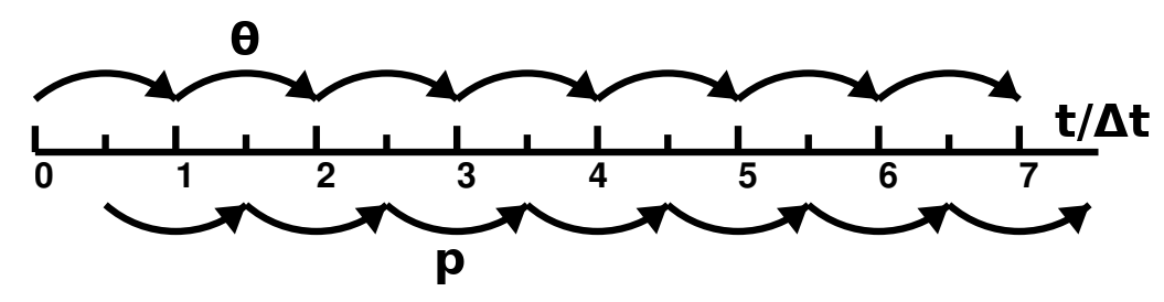
Analogy of Pendulum with Accelerator
Phase focusing with rf cavities:
- particles drift over most of the circular accelerator
- particles get kicked only in rf cavities
(energy change through standing electromagnetic wave)
$\implies$ closely corresponds to discrete pendulum situation!
Summary
- time scales in accelerator physics
- phase space & Hamiltonian functional
- discrete numerical integration schemes:
- Euler
- Euler-Cromer
- Leapfrog
- symplecticity
Literature:
- symplectic integrators: https://young.physics.ucsc.edu/115/leapfrog.pdf