Numerical Methods of Accelerator Physics
Lecture by Dr. Adrian Oeftiger

Part 12: 27.01.2023
Run this notebook online!
Interact and run this jupyter notebook online:
![]()
$\implies$ make sure you installed all the required python packages (see the README)!
Finally, also find this lecture rendered as HTML slides on github $\nearrow$ along with the source repository $\nearrow$.
Run this first!
Imports and modules:
from config import (np, plt, tqdm, trange, c, epsilon_0,
                    beta, gamma, Machine, track_one_turn,
                    charge, mass, emittance, hamiltonian, U,
                    plot_hamiltonian, plot_rf_overview,
                    plot_dist)
%matplotlib inline
If the progress bar by tqdm (trange) in this document does not work, run this:
!jupyter nbextension enable --py widgetsnbextension
Enabling notebook extension jupyter-js-widgets/extension...
      - Validating: OK
Refresher!
- reinforcement learning: solve decision-making problems, optimise for best behavior in an environment
- Markov decision process: state, action, probability, reward
- Q-learning with state-action value function $Q(s,a)$
- temporal difference rule, learning rate
- policy: optimal policy via acting greedily in terms of $Q$
- Q-learning:
- Lookup table: discrete state-action spaces
- Q-net (neural network): continuous states, discrete action space
- Actor-critic methods evolve from Q-learning and use two networks:
- One for the policy (actor) and one to estimate the Q-values (critic)
- continuous states and actions.
Today!
- Intro Collective Effects
- Space-charge Modelling
- Negative-Mass / Microwave Instability
Part I: Intro Collective Effects
Reminder: What is an "accelerator"?
$$\begin{array}\,\text{beam self fields} &>& \text{external applied fields} &\text{(plasma)} \\ \text{beam self fields} &\ll& \text{external applied fields}& \text{(accelerator)}\end{array}$$$\implies$ perturbation technique applicable to higher-energy accelerators:
$$\begin{cases} \text{unperturbed motion} &=& \text{external fields} \\ \text{perturbation} &=& \text{self fields} \end{cases}$$Large part of this course: model effects on particle beam due to external fields!
Main collective effects
Beam dynamics due to intensity and beam fields $=$ "collective effects"
- Coulomb repulsion between beam particles:
- space charge (mean-field effect)
- intra-beam scattering (collision effect)
- beam interaction with induced currents in metallic environment
- beam-coupling impedance
- beam interaction with rest gas:
- electron cloud instability (ion + positron beams)
- fast beam-ion instability (electron beams)
- beam-beam interaction (colliders)
Part II: Space-charge Modelling
Paraxial Approximation
In synchrotrons: weak relative motion of particles within bunch vs. motion of entire bunch
$$p_x,p_y \ll p_0 \qquad \text{and} \qquad \delta \ll 1$$$\implies$ for space charge: relative motion between particles can be neglected!
Approach
Approach to modelling space-charge in synchrotrons:
- neglect relative motion $\implies$ no magnetic fields in beam reference frame
- solve electrostatic problem of charged particle distribution $\rho$ via Poisson equation
$\quad~$ to obtain self (or space-charge) fields
$$\mathbf{E}_\mathrm{sc}=-\nabla \varphi$$- (Lorentz) transform self fields from beam to laboratory reference frame
- add self fields to external (magnetic & rf) fields, apply to solve for particle motion
(typical method: alternate transport maps and integrated collective effects kicks)
Space-charge Forces
The magnetic fields in the lab frame purely come from the Lorentz transform of the electric field:
$$(B_x, B_y, B_z)_\mathrm{lab} = \left(-\frac{\beta E_y}{c}, \frac{\beta E_x}{c}, 0\right)_\mathrm{lab}$$(if avoiding Lorentz transforms, one can also derive this result from Faraday's induction law!)
With $\mathbf{v}=\beta c \hat{\mathbf{e}}_z$, the Lorentz force $\mathbf{F}=q(\mathbf{E} + \mathbf{v}\times\mathbf{B})$ effectively leads to a cancellation of electric and magnetic forces with a factor $1-\beta^2$ in the transverse plane!
The space-charge force on a particle of charge $q$ in lab frame reads:
$$\begin{align} (F_x, F_y, F_z)_\mathrm{lab} &= q\left((1 - \beta^2)E_x, (1 - \beta^2)E_y, E_z\right)_\mathrm{lab}\\ &= q\left(\frac{E_x}{\gamma^2}, \frac{E_y}{\gamma^2}, E_z\right)_\mathrm{lab} \end{align}$$$\implies$ transverse space-charge forces reduce with energy by $1/\gamma^2$, that is, most important at injection energy and for ion beams!
Transverse Space Charge
The transverse space-charge force enters the Hill equation, which governs the evolution of single particles:
$$\begin{align} \cfrac{d^2x}{ds^2} + \left(\cfrac{1}{\rho_0(s)^2} + k(s)\right) x &= \cfrac{F_x(x,y)}{p_0\beta c} \\ \cfrac{d^2y}{ds^2} -k(s) y &= \cfrac{F_y(x,y)}{p_0\beta c} \end{align}$$Remarks:
- transverse degrees of freedom are generally coupled by space-charge force
- transverse space charge counteracts external focusing and leads to negative tune shifts
(easy to see: plug in a linear $E_r \propto \frac{r}{r_b^2}$ for $r_b$ the beam radius)
Longitudinal Space Charge

Ion bunch lengths (meters) usually exceed beam pipe radius (centimeters)!
In perfectly conducting beam pipe, field lines end perpendicular in wall!
$\implies$ longitudinal space-charge model:
- differs from free-space solution and
- depends on ratio between transverse beam size $r_b$ and pipe radius $r_p$
image from M. Reiser
Simplistic Derivation of $\lambda'$ Model
Consider a round continuous beam of radius $r_b$ in cylindrical vacuum pipe of radius $r_p$:
- beam (particles) velocity: $\beta c$
- line charge density (Coulomb per meter): $\lambda(z)$
$$\oint \mathbf{E}\cdot \mathbf{dl} = - \frac{\partial}{\partial t} \iint_S \mathbf{B}\cdot\mathbf{dS}$$
Choose rectangle as follows for circular path $\mathbf{l}$ with a small $\Delta z\rightarrow dz$:
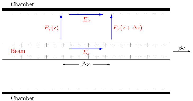
image from C. Prior
Faraday's law: set $\mathrm{LHS}=\mathrm{RHS}$, replace $\frac{\lambda(z+\Delta z) - \lambda(z)}{\Delta z}\approx \frac{d\lambda(z)}{dz}$ and find
$$\implies E_z(z) = E_w - \frac{1}{4\pi\epsilon_0}\underbrace{\left(1 + 2\ln\cfrac{r_p}{r_b}\right)}\limits_{\mathop{\doteq} g} \, \underbrace{(1-\beta^2)}\limits_{\mathop{=}\frac{1}{\gamma^2}} \, \cfrac{d\lambda}{dz}$$Longitudinal Space-charge Field
geometry factor $g$ $\implies$ represents field line distortion with $r_p/r_b$ ratio!
$\implies$ $E_z$ expression includes both direct and indirect space-charge contributions.
For perfectly conducting walls the electric field in the wall vanishes, $E_w=0$.
$\implies$ Note that also longitudinal space charge reduces with $1/\gamma^2$ for fixed bunch length!
The $\lambda'$ Space-charge Model
For typically slow synchrotron motion, the particles do not move much, $z\approx\mathrm{const}$ during a turn. Evaluate longitudinal space-charge effect with a single kick per turn approximating $F_z(z)=q E_z(z)=\mathrm{const}$ during the revolution.
Momentum update according to the $\lambda'$ space-charge model thus reads:
$$\Delta p_{n+1} = \Delta p_n - \frac{qg}{4\pi\epsilon_0\gamma^2} \frac{C}{\beta c}\frac{d\lambda}{dz}$$$\implies$ Self-consistent modelling: feedback due to macro-particle distribution determining the space-charge field which is in turn applied to the macro-particles!
Derived $\lambda'(z)$ space-charge model for continuous beam, but it also applies to long bunches with the condition:
$$\sigma_z \gtrsim 3 r_p$$NB: this longitudinal $\lambda'$ space-charge model (for perfectly conducting boundaries) is equivalent to a constant impedance model with a negative inductance ($Z\propto -iL$)
Example: Longitudinal Space Charge in CERN PS
Consider CERN PS for illustration once again:
- non-accelerating rf bucket at $V_\mathrm{RF}=25\,$kV
- injection energy $\gamma=3.13$
- bunch of $N_p = 1\times 10^{12}$ particles
- rms bunch length of $\sigma_z=2\,$m
- vacuum pipe of $\approx 10\,$cm
- beam radius of $\approx 1\,$cm
m = Machine(gamma_ref=3.13, phi_s=0, voltage=25000)
# adjust here later!
The RF harmonic determines the width of an RF bucket:
m.harmonic
7
$\implies$ Can you determine the location of the left and right unstable fix points, which limit the RF bucket?
rfbucket_z_right = # fill me
rfbucket_z_left = # fill me
plot_rf_overview(m);

We initialise a Gaussian bunch distribution with small rms bunch length $\sigma_z=2\,$m (so that the small-amplitude approximation applies):
sigma_z = 2
$\implies$ Is the bunch length condition for our $\lambda'(z)$ longitudinal space-charge model satisfied?
The matched rms momentum spread $\sigma_{\Delta p}$ (remember, $\sigma_{\Delta p}$ and $\sigma_z$ are linked via equal Hamiltonian values $\mathcal{H}_0$, the equilibrium condition):
sigma_deltap = np.sqrt(
    2 * m.p0() / np.abs(m.eta(0)) *
    charge * m.voltage * np.pi * m.harmonic / (beta(gamma(m.p0())) * c * m.circumference**2)
) * sigma_z
sigma_deltap / m.p0()
0.000512530680190112
Number of simulated macro-particles (not too low such as to well resolve the line charge density of the bunch):
N = 100000
Generation of macro-particles by initialising the phase-space distribution:
np.random.seed(12345)

z = np.random.normal(loc=0, scale=sigma_z, size=N)
deltap = np.random.normal(loc=0, scale=sigma_deltap, size=N)
plot_hamiltonian(m, dpmax=0.005)
plt.scatter(z[::N // 1000], deltap[::N // 1000] / m.p0(), marker='.', s=1);

$\implies$ Does this generated macro-particle distribution appear to be matched to the RF bucket?
Next, we define a regular 1D grid for discretisation -- we will slice up the beam into bins (the slices):
N_slices = 100

slice_boundaries = np.linspace(rfbucket_z_left, rfbucket_z_right, N_slices + 1, endpoint=True)
slice_centres = (slice_boundaries[1:] + slice_boundaries[:-1]) / 2
And we are now in the position to compute a discretised line charge density $\lambda(z)$ from the $z$ distribution of the macro-particles:
N_per_slice, slice_boundaries = np.histogram(z, bins=slice_boundaries)
plt.step(slice_centres, N_per_slice, where='mid')
plt.xlabel('$z$ [m]')
plt.ylabel('Number of particles / slice');

The bunch has a total intensity of $N_p=1\times 10^{12}$ real particles.
$\implies$ What total charge does a macro-particle carry?
charge_per_mp = 1e12 / N * charge
lmbda = charge_per_mp * N_per_slice / np.diff(slice_boundaries)
We evaluate the geometry factor $g$:
r_pipe = 0.1
r_beam = 0.01

g = 1 + 2 * np.log(r_pipe / r_beam)
If the space-charge field is given by $E_z\propto \frac{d\lambda}{dz}$, the space-charge potential is given by the same expression but with $V_\mathrm{sc} \propto -\lambda$!
V_sc = g / (4 * np.pi * epsilon_0 * m.gamma_ref**2) * lmbda
plt.plot(slice_centres, V_sc)
plt.xlabel('$z$ [m]')
plt.ylabel('$|V_{sc}|$ [V]');

$\implies$ Compare this space-charge potential to the rf voltage – what do you think about the peak values?
Compute the derivative of the line charge density via second-order (symmetric) finite difference,
$$\lambda'(z)\approx \cfrac{\lambda(z+\Delta z) - \lambda(z-\Delta z)}{2\Delta z} \quad:$$lmbda_prime = np.gradient(lmbda, slice_centres)
plt.step(slice_centres, 1e9 * lmbda_prime)
plt.xlabel('$z$ [m]')
plt.ylabel("$\lambda'(z)$ [nC/m${}^2$]");

The longitudinal space-charge field is thus given by:
E_z = -g / (4 * np.pi * epsilon_0 * m.gamma_ref**2) * lmbda_prime
Comparison with external phase focusing from RF
Compute the effective external RF field as a mean via the rf wave kick per circumference:
E_rf = m.voltage / m.circumference * np.sin(
    -m.harmonic * slice_centres * 2 * np.pi / m.circumference + m.phi_s)
# E_rf = -np.gradient(U(slice_centres, m) / charge * c, slice_centres)
The external phase focusing by the rf wave and the space-charge field sum up:
plt.plot(slice_centres, E_rf, c='k', label='RF')
plt.plot(slice_centres, E_z, c='r', label='SC')
plt.plot(slice_centres, E_rf + E_z, c='lightblue', label='RF+SC')

plt.legend()
plt.xlabel('$z$ [m]')
plt.ylabel('mean $E$ [V/m]');

$\implies$ What happens to the net phase focusing which the bunch experiences? Will the RF bucket increase or rather shrink in momentum acceptance?
Longitudinal Space Charge vs. Transition
Since the chosen flank (falling/rising) of the rf wave depends on the phase slippage (below/above transition), the effect of longitudinal space charge on phase focusing depends on classical vs. relativistic regime!
| classical regime | relativistic regime |
|---|---|
| $\eta < 0$ | $ \eta > 0$ |
| $\gamma < \gamma_\text{t}$ | $\gamma > \gamma_\text{t}$ |
| $\implies$ $\varphi_s$ on rising slope of $V(\varphi)$ | $\implies$ $\varphi_s$ on falling slope of $V(\varphi)$ |
| [$z(\varphi_s)$ on falling slope of $V(z)$] | [$z(\varphi_s)$ on rising slope of $V(z)$] |
| space charge defocuses | space charge focuses |
$\implies$ Choose $\gamma=7$. Are we above transition energy? Provide stable rf conditions and repeat the above computations! Can you confirm that space charge acts in the same way (focusing) as the rf wave now?
Fate of a Perturbation?
Consider a (space-charge-) matched distribution in longitudinal phase space. Suppose a small perturbation in the line charge density, e.g. a trough in the bunch profile. The effect by the space-charge field:
$$E_z(z) = -\cfrac{g}{4\pi\epsilon_0\gamma^2}\,\cfrac{d\lambda}{dz}$$- below transition:
- particles speed up in regions where $\frac{d\lambda}{dz}<0$
- particles slow down in regions where $\frac{d\lambda}{dz}>0$
$\implies$ the trough will be filled with particles, the perturbation is damped
- above transition: reverse situation!
$\implies$ the perturbation grows
$\implies$ INSTABILITY!
Part III: Negative-Mass / Microwave Instability
About the Microwave Instability
- instability typically develops above intensity threshold
- instability only appears above transition
- often observed as bunch length oscillations increasing on average, immediately after transition crossing $\implies$ longitudinal emittance growth
- emittance growth leads to larger synchrotron tune spread $\implies$ eventual Landau damping of instability (natural end of instability evolution)
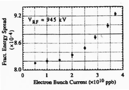
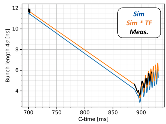
images from E. Shaposhnikova and A. Lasheen
Let's simulate it!
We implement the space-charge kick for the tracking:
def space_charge_kick(z_n, deltap_n, machine, charge_per_mp=charge_per_mp, N_slices=N_slices, g=g):
    m = machine
    rfbucket_z_right = m.circumference / m.harmonic / 2
    rfbucket_z_left = -rfbucket_z_right

    # slicing
    slice_boundaries = np.linspace(rfbucket_z_left, rfbucket_z_right, N_slices + 1, endpoint=True)
    N_per_slice, _ = np.histogram(z_n, bins=slice_boundaries)
    # find slice index for each particle:
    slice_idx_per_mp = np.floor((z_n - slice_boundaries[0]) /
                                (slice_boundaries[1] - slice_boundaries[0])).astype(int)

    # get line charge density derivative
    lmbda = charge_per_mp * N_per_slice / np.diff(slice_boundaries)
    lmbda_prime = np.gradient(lmbda, slice_boundaries[:-1])

    # space-charge field per slice
    E_z = -g / (4 * np.pi * epsilon_0 * m.gamma_ref**2) * lmbda_prime

    # momentum update
    deltap_n1 = deltap_n - charge * E_z[slice_idx_per_mp] * m.circumference / (beta(m.gamma_ref) * c)
    return deltap_n1
The kicks which the particles receive look as follows:
plt.scatter(z, (space_charge_kick(z, deltap, m) - deltap) / m.p0())
plt.xlabel('$z$ [m]')
plt.ylabel('$(\Delta p_{n+1} - \Delta p_{n}) / p_0$');

We implement the one-turn tracking:
def track_one_turn(z_n, deltap_n, machine, **kwargs):
    m = machine
    # half drift
    z_nhalf = z_n - m.eta(deltap_n) * deltap_n / m.p0() * m.circumference / 2
    # rf kick
    amplitude = charge * m.voltage / (beta(gamma(m.p0())) * c)
    phi = m.phi_s - m.harmonic * 2 * np.pi * z_nhalf / m.circumference

    m.update_gamma_ref()
    deltap_n1 = deltap_n + amplitude * (np.sin(phi) - np.sin(m.phi_s))
    # space-charge kick
    deltap_n1 = space_charge_kick(z, deltap_n1, m, **kwargs)
    # half drift
    z_n1 = z_nhalf - m.eta(deltap_n1) * deltap_n1 / m.p0() * m.circumference / 2
    return z_n1, deltap_n1
Ready to Simulate!
We simulate just above transition, continuing from the end of the previous part.
assert m.gamma_ref > 1 / np.sqrt(m.alpha_c), 'Initialise the machine above transition energy!'
We simulate for a bit more than 1 synchrotron period above transition at 10x higher intensity than the initial nominal parameters:
n_turns = 3000

intensity_factor = 10
... and record the longitudinal emittance:
epsn_z = np.zeros(n_turns, dtype=np.float64)

epsn_z[0] = emittance(z, deltap)
... as well as the bunch profiles (just as we did in the tomography lecture 09):
profiles = [np.histogram(z, bins=slice_boundaries)[0]]
Let's track! (May take a couple of minutes!)
for i_turn in trange(1, n_turns):
    z, deltap = track_one_turn(z, deltap, m,
                               charge_per_mp=charge_per_mp * intensity_factor,
                               N_slices=400)

    # record:
    epsn_z[i_turn] = emittance(z, deltap)
    profiles += [np.histogram(z, bins=slice_boundaries)[0]]
0%| | 0/9999 [00:00<?, ?it/s]
Let us have a look at the final bunch profile:
N_per_slice, slice_boundaries = np.histogram(z, bins=slice_boundaries)

plt.step(slice_centres, N_per_slice, where='mid')
plt.xlabel('$z$ [m]')
plt.ylabel('Number of particles / slice');

$\implies$ we note distinct peaks (enhanced perturbations) along the bunch profile!
Let's plot the emittance evolution:
plt.plot(np.arange(n_turns), 100 * (epsn_z - epsn_z[0]) / epsn_z[0])

plt.xlabel('Turns')
plt.ylabel('$\Delta \epsilon_z/\epsilon_{z0}$ [%]');

$\implies$ there is strong emittance blow-up for 10x higher intensity! (Does this persist for nominal intensity?)
Look into phase space and a couple of particles:
plot_hamiltonian(m, dpmax=0.005)
plt.scatter(z[::N // 1000], deltap[::N // 1000] / m.p0(), marker='.', s=1);

A density plot of the longitudinal phase space shows the damage:
plt.hist2d(z, deltap/m.p0(), bins=100)

plt.xlabel('$z$ [m]')
plt.ylabel('$\delta$');

And the bunch profiles over time:
plt.imshow(profiles, origin='lower', cmap='jet', extent=(rfbucket_z_left, rfbucket_z_right, 0, n_turns))
plt.gca().set_aspect(np.diff(plt.xlim()) / np.diff(plt.ylim()))
plt.xlabel('$z$ [m]')
plt.ylabel('Turn')
plt.colorbar(label='Density');

$\implies$ there is a clear signature for the microwave instability: look at the diverging distribution and the high-frequency structure of space-charge waves on the profiles!
$\implies$ If you go for the original proton beam intensity, will the instability persist? Change the intensity_factor from 10.0 (back) to 1.0 and re-run the entire notebook (to re-initialise the macro-particle distribution).
Actual CERN PS Measurements
A recent paper from CERN shows real measurements from the CERN PS:
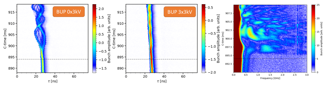
image from A. Lasheen
$\implies$ note the activity in the GHz range due to the enhancing perturbations (hence the name microwave instability)
Summary
- collective effects: direct Coulomb repulsion, indirect wall effects, vacuum effects, beam-beam interaction
- transverse space charge: defocusing
- $\lambda'(z)$ model for longitudinal space charge
- longitudinal space charge: defocusing below transition, focusing above transition
- microwave instability: destroys longitudinal bunch structure
(high-frequency space-charge waves, enhancing of perturbations)
Literature
- Martin Reiser, Theory and Design of Charged Particle Beams, Chapter 5.4 (.7-.9 for longitudinal space-charge dynamics)
- Elena Shaposhnikova, Signatures of Microwave Instability