Numerical Methods of Accelerator Physics

Lecture by Dr. Adrian Oeftiger

Part 4: 18.11.2022

Run this notebook online!

Interact and run this jupyter notebook online:

1. via the public mybinder.org service:

2. on the local TU Darmstadt jupyterhub $\nearrow$ (using your TU ID)

$\implies$ make sure you installed all the required python packages (see the README)!

Finally, also find this lecture rendered as HTML slides on github $\nearrow$ along with the source repository $\nearrow$.

Refresher!

• sources for non-linearities in accelerators
• deterministic chaos: (bounded) deterministic dynamics with a positive Lyapunov exponent
  • sensitivity to initial conditions
  • cannot reliably compute prediction for long-term time scales
• early indicators of chaotic motion:
  • (maximum) Lyapunov exponent
  • frequency diffusion via Frequency Map Analysis (FMA), employing the NAFF algorithm
• numerical artefacts: rounding and truncation, machine precision

Today!

1. Acceleration with RF Cavities
2. Longitudinal Beam Dynamics (Tracking Equations)

A Relativistic Particle

Relativistic particle of rest mass $m_0$ at velocity $\mathbf{v}$ features momentum

$$p=|\mathbf{p}|=|\gamma m_0 \mathbf{v}| = \gamma m_0 \beta c$$

where

$$\begin{align} c&\text{: speed of light in vacuum,}\qquad &c&\doteq 2.998\times 10^8 \text{m/s} \\ \beta&\text{: particle speed in units of }c,\qquad&\beta&\doteq |\mathbf{v}/c| < 1 \\ \gamma&\text{: relativistic Lorentz factor,}\qquad &\gamma&\doteq\cfrac{1}{\sqrt{1 - \beta^2}} > 1 \end{align}$$

Total energy defined by

$$E_\text{tot}=\gamma m_0 c^2$$

and related to momentum $p$ by the relativistic equation

$$E_\text{tot}^2=\bigl(m_0c^2\bigr)^2 + (pc)^2$$

Lorentz Force

Utilise electromagnetic fields $(\mathbf{E},\mathbf{B})$ to exert Lorentz force $\mathbf{F}_L$ on particle of charge $q$:

$$\frac{d\mathbf{p}}{dt} = \mathbf{F} = q\,(\mathbf{E}+\mathbf{v}\times\mathbf{B})$$

Deriving relativistic equation by time $t$ and using definition of $E_\text{tot}$:

$$\implies E_\text{tot} \frac{dE_\text{tot}}{dt} = c^2\cdot\mathbf{p}\cdot \frac{d\mathbf{p}}{dt} = c^2\cdot \mathbf{p}\cdot\mathbf{F}_L$$$$\stackrel{/E_\text{tot}}{\implies} \frac{dE_\text{tot}}{dt} = \mathbf{v}\cdot\mathbf{F}_L = q\cdot \mathbf{v}\cdot(\mathbf{E}+\underbrace{\mathbf{v}\times \mathbf{B}}\limits_\text{cancels}) = q\cdot \mathbf{v}\cdot\mathbf{E}$$

i.e. the total energy can only be increased by electric field components!

How to Accelerate?

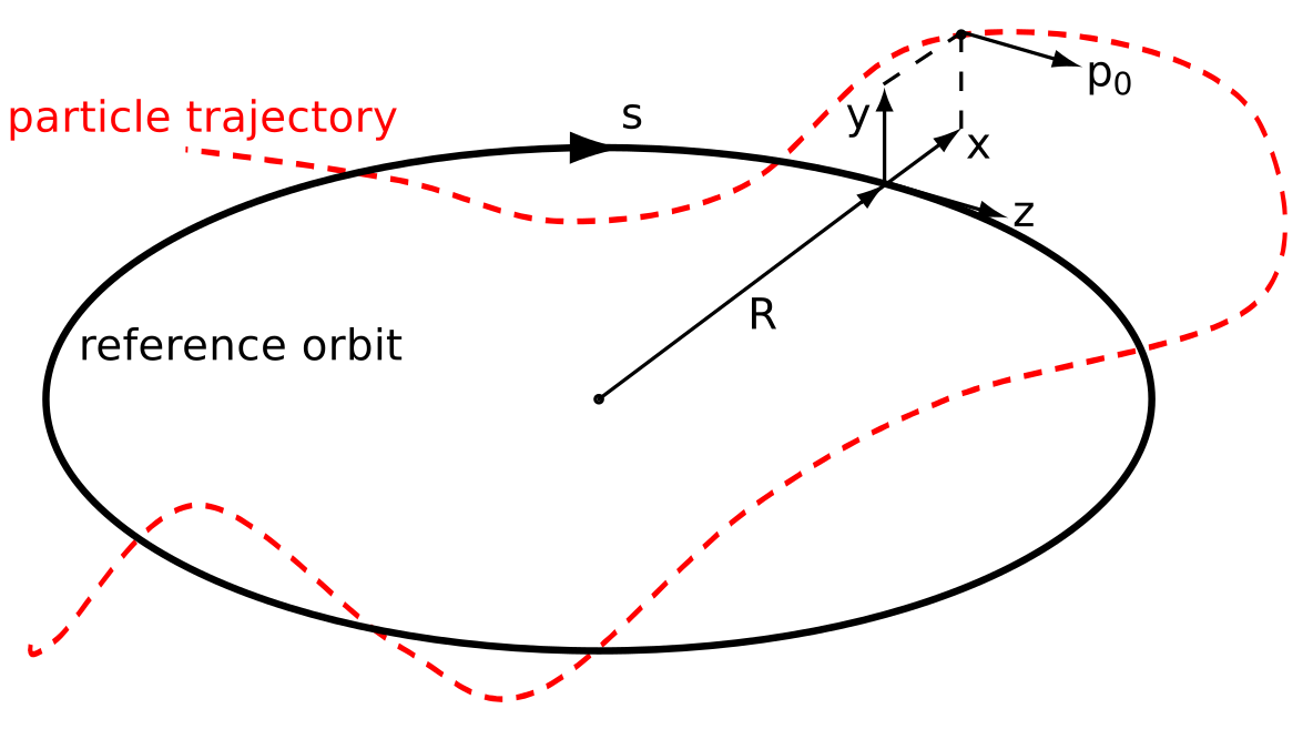
Particle moves along path length $s$ with velocity

$$\mathbf{v}_s = \frac{d\mathbf{s}}{dt}$$

Variation of particle energy along $s$ ("$\approx$"$\rightarrow$ paraxial approximation):

$$\implies \frac{dE_\mathrm{tot}}{ds} = \frac{1}{v_s} \frac{dE_\mathrm{tot}}{dt} = q \cdot \frac{\mathbf{v}}{v_s}\cdot \mathbf{E} = q \cdot \Bigl(\underbrace{\frac{v_z}{v_s}}\limits_{\mathop{\approx}1}E_z + \underbrace{\frac{v_x}{v_s}}\limits_{\mathop{\approx}\frac{dx}{ds}\mathop{\equiv}x'}\cdot E_x + \underbrace{\frac{v_y}{v_s}}\limits_{\mathop{\approx}\frac{dy}{ds}\mathop{\equiv}y'}\cdot E_y \Bigr)$$$$\implies\left\{\begin{array}\, x',~y'&\text{: transverse momenta or slopes, small }\leftrightarrow\text{transverse electric fields have weak impact} \\ E_z&\text{ : longitudinal electric field most efficient to provide }\cfrac{dE_\mathrm{tot}}{ds} \end{array}\right.$$

Accelerate!

3 typical ways to supply $E_z$:

1. DC field (single passage!)

   • electrostatic accelerators: few MV/m before breakdown
   • plasma accelerators: more than 100 GV/m

2. AC field: travelling wave rf cavities
   $\rightarrow$ ultra-relativistic particles (typically electrons)

3. AC field: resonator / standing wave rf cavities:
   $\rightarrow$ most versatile standard (International Linear Collider project: 35 MV/m)

Part I: Momentum / Energy Gain

Longitudinal phase space: $(z, {\color{red}{\delta}})$

RF Resonator: Modes

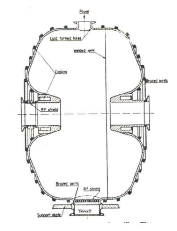
Particles travel through rf cavity in vacuum: piece of metal enclosing an empty volume!

$\implies$ boundary conditions $\leftrightarrow$ electromagnetic discrete solutions $\mathbf{E}_n(\mathbf{r})$ to Maxwell equations, resonating modes!

Each resonating mode identified by index $n$, characterised by field amplitude maps $\mathbf{E}_n(\mathbf{r}),\mathbf{B}_n(\mathbf{r})$ and oscillating at RF frequency $f_n=\omega_n/2\pi$!

$\mathbf{E}_n$ satisfies the boundary conditions! At given time $t$, total electric field in cavity given by:

$$\mathbf{E}(\mathbf{r}, t) = \sum\limits_{n} e_n(t) \cdot \mathbf{E}_n(\mathbf{r})$$

where $e_n(t)$ is the field time variation (can be modelled by RLC circuit i.e. damped harmonic oscillator equation).

image from B. Holzer

RF Resonator: Maxwell Equations

Often use Finite Integration Technique (cf. other lectures) to compute $\mathbf{E}_n(\mathbf{r}),\mathbf{B}_n(\mathbf{r})$ for given rf cavity geometry based on Maxwell equations:

$$\left\{\begin{array}\, \nabla \cdot \mathbf{E} &= \frac{\rho}{\epsilon_0} \\ \nabla \times \mathbf{E} + \frac{\partial\mathbf{B}}{\partial t} &= \mathbf{0} \\ \nabla \cdot \mathbf{B} &= 0 \\ \nabla \times \mathbf{B} - \frac{1}{c^2} \frac{\partial\mathbf{E}}{\partial t} &= \mu_0 \mathbf{j} \end{array}\right\} \quad\text{with bound. cond.}\quad \left\{\begin{array}\, \mathbf{n}\cdot \mathbf{E}_n &= \frac{\sigma}{\epsilon_0} \\ \mathbf{n}\times \mathbf{E}_n &= \mathbf{0} \\ \mathbf{n}\cdot \mathbf{B} &= 0 \\ \mathbf{n}\times (\mu\cdot\mathbf{B}_n) &= \mathbf{K} \end{array}\right\}$$

where $\mathbf{n}$ is normal to the conductor surface, $\sigma$ the charge surface density and $\mathbf{K}$ the current surface density.

$\implies$ choose one $\mathbf{E}_n$ as accelerating mode with optimal $E_z$ component along cavity axis (often TM${}_{010}$), optimise cavity geometry, mode is excited by injecting rf power via coupler!

image from J. Le Duff

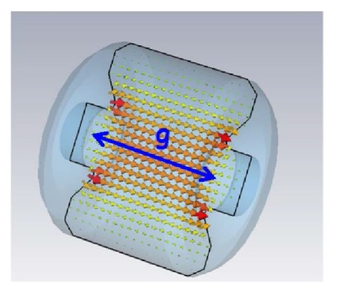
Transit-time Factor

Consider only accelerating mode excited in cavity. Particle travelling along cavity axis $s$ while time $t$ passes:

$$E_z(s, t) = E_{z,0}(s) \cdot \sin\bigl(\omega_\text{rf}\, t + \varphi_s\bigr)$$

Here, $\varphi_s$ refers to synchronous phase at arrival of "synchronous" reference particle. Total cavity voltage is given by:

$$V_0 = \int\limits_{-\infty}^{+\infty} ds\cdot|E_{z,0}(s)|$$

Hypothetical maximum energy gain is $\Delta W = |q|\cdot V_0$ for particle of charge $q$.

$\implies$ Real $\Delta W$ reduces due to inevitable field variation during gap transit. Transit-time factor:

$$ T = \frac{\text{energy gain of particle with }v=\beta c}{\text{maximum energy gain (particle with }v\rightarrow\infty\text{)}} \leq 1 $$

Approximation #1: Velocity Change

A priori, energy gain is associated with particle velocity change, i.e. exact $T$ depends on $d\beta$ during passage through rf cavity.

For synchrotrons, effect of velocity change is typically negligible to determine energy gain ($\Delta W\propto\Delta\gamma$):

$$\frac{d\beta}{\beta} = \frac{1}{\beta^2\gamma^2} \cdot \frac{d\gamma}{\gamma}$$

$\implies$ two scenarios where approximation of $T$ independence of $\Delta\beta$ applies:

$$\left\{\begin{array}\, \gamma \gg 1 &\text{: particle is already ultra-relativistic} \\ \Delta\gamma \ll \beta\gamma &\text{: energy gain in cavity is much smaller than particle momentum} \end{array}\right.$$

Simple Example for $T$

Consider uniform standing wave with $E_{z,0}(s)=V_0/g=\mathrm{const}$ across gap width $g$ (zero field outside), at crest of rf wave, i.e. $\varphi_s=\pi/2$:

$$E_z(s, t) = \frac{V_0}{g} \,\cos(\omega_\text{rf}\,t)$$

The synchronous particle travels along $s=\beta c t$ (assuming constant $v=\beta c$) and picks up an actual maximum energy gain

$$\implies \Delta W = \cfrac{q V_0}{g}\int\limits_{-g/2}^{+g/2} ds\cdot \cos\left(\cfrac{\omega_\text{rf}\,s}{\beta c}\right)$$

and the transit-time factor becomes:

$$T = \left| \cfrac{\sin\left(\cfrac{\omega_\text{rf} g}{2\beta c}\right)}{\cfrac{\omega_\text{rf} g}{2\beta c}} \right| \quad \implies\quad T\rightarrow 1 \Leftrightarrow \left\{\begin{array}\, g \rightarrow 0 \\ \omega_\text{rf} \rightarrow 0 \\ \beta c \rightarrow \infty \end{array}\right.$$

$\implies$ reduction in effective energy gain ($T<1$) is mostly relevant for low-energy protons and ions!

Energy Gain by RF Cavity

Design / reference energy increases as determined by synchronous phase $\varphi_s$,

$$\Delta W_0 = q V\cdot\sin(\varphi_s)$$

with the effective rf voltage $V = V_0 T$.

Real particles travel at a longitudinal distance $z = s - \beta c t$ to synchronous particle. They experience the rf kick at phase $\varphi = \omega_\text{rf}\,t = \varphi_s - \cfrac{\omega_\text{rf} z}{\beta c}$. Corresponding energy gain is $\Delta W = q V\cdot \sin(\varphi)$.

Expressed as an energy distance $\Delta E$ to the synchronous particle, $\Delta E=E_\text{tot} - E_{\text{tot},0}$, the discrete energy update of an arbitrary particle passing through an rf cavity becomes

$$\begin{align} \Delta E|_\text{after} &= \Delta E|_\text{before} + \Delta W - \Delta W_0 \\ &= \Delta E|_\text{before} + q V\cdot \bigl(\sin(\varphi) - \sin(\varphi_s)\bigr) \end{align}$$

from config import np, plt, plot_rfwave
from scipy.constants import m_p, e, c
%matplotlib inline

Phase Focusing Effect

$$\Delta E|_\text{after} = \Delta E|_\text{before} + q V\cdot \left(\sin\left(\varphi_s - \frac{\omega_\text{rf}z}{\beta c}\right) - \sin(\varphi_s)\right)$$

Phase focusing principle (classical regime):

• particle with $\varphi>\varphi_s$ arrives later and has $\color{blue}{\delta < 0}$: accelerated towards synchronous particle!
• particle with $\varphi<\varphi_s$ arrives early and has $\color{orange}{\delta > 0}$: decelerated towards synchronous particle!

plot_rfwave();

Earnshaw's Theorem

"A charged body cannot be held in stable equilibrium by electrostatic forces from other charged bodies."

S. Earnshaw (1839), Trans. Camb. Phil. Soc. 7 97

$\implies$ application to rf accelerators: always one direction in 3D which is defocused!

Approximation #2: Transverse Defocusing

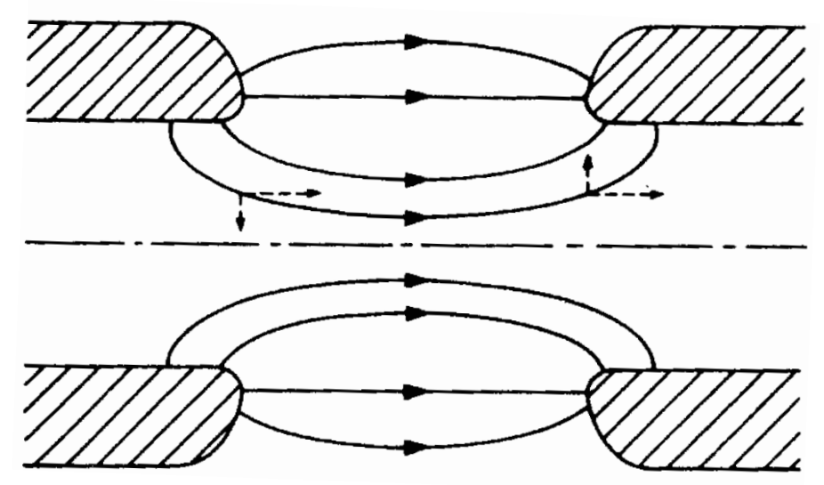
Real $\mathbf{E}$ field across gap in rf cavities has transverse component when off axis, classical regime:

• focusing at entry
• defocusing at exit

$\implies$ DC field leads to net focusing effect (due to gain in longitudinal momentum), but AC field in case of stable longitudinal motion: net defocusing effect (rise in voltage during passage)

$\implies$ typically very weak vs. quadrupole fields and hence often neglected for synchrotrons

Beam rigidity

Constant dipole field $B$ to steer reference particle around corner at bending radius $\rho$:

$$\begin{align} F_\text{centrip} &= F_\text{L} \\ \frac{\gamma m_0 v^2}{\rho} &= |q| v B \end{align}$$

$$\implies B\rho = \cfrac{p}{|q|}$$

"Beam rigidity"

Synchrotron

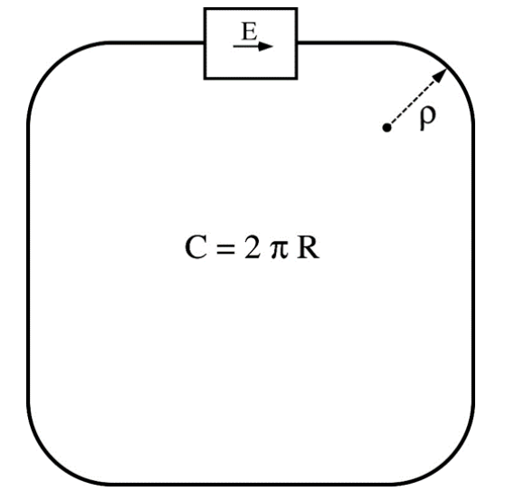
A synchrotron:

• is a ring with a constant reference orbit of circumference $C$,
  determined by the dipole magnets (defining the beam rigidity)
• has rf systems powered at revolution frequency $f_\text{rev}$
  or integer multiple of it ("harmonic" $h$): synchronisation!

$$\begin{align} f_\text{rev} &= \frac{\beta c}{C} \\ f_\text{rf} &= h\,f_\text{rev} \end{align}$$

$\implies$ $h$ synchronous particles moving on reference orbit! To accelerate them and for longitudinal phase focusing around them, apply $E_z$ in rf cavity!

$\implies$ only works with AC field! Why not DC field across cavity gap?

image from A. Chance and N. Pichoff

Acceleration in Synchrotron

Require dipole fields to align with increasing momentum to maintain synchronicity!

$$\dot{B}=\frac{\dot{p}}{|q|\rho}$$

$\implies$ "cycle": synchrotrons ramp up magnets for acceleration (and back down to receive next beam for acceleration)

Part II: Longitudinal Drift

Longitudinal phase space: $({\color{red}{z}}, \delta)$

Mechanism behind Synchrotron

Conceptual "flow chart" of synchrotron operation principle:

1. dipole field $B$ increase
2. thus, bending radius $\rho$ decrease
3. thus, reference orbit length decrease
4. thus, synchronous phase $\varphi_s$ decrease (earlier arrival of synchronous particle)
5. thus, reference energy/momentum increase (if sufficient rf voltage)
6. thus, back to synchronism (possibly shorter equilibrium reference orbit)

$\implies$ typically magnetic field ramp $\dot{B}$ is slow enough $\implies$ adiabatic acceleration, particles remain focused around synchronous particle

Off-momentum Trajectory

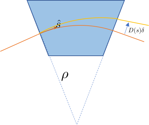
image from Y. Hao

Particles with higher momentum $\delta = \Delta p/p > 0$ than the reference particle are bent less (larger $p$ $\implies$ larger $\rho$)!

$$\implies d\ell = \left(1 + \frac{x}{\rho(s)}\right) ds$$

$\implies$ larger equilibrium orbit around the machine for fixed dipole fields $B$!

Can describe this horizontal offset $x$ due to momentum offset $\delta$ by dispersion function $D_x(s)$ (more details later in transverse dynamics lecture):

$$x(s) = D_x(s) \delta$$

Integrating around machine to get full orbit length:

$$\ell_\text{tot} = \oint d\ell = \underbrace{\oint ds}\limits_{\mathop{\equiv} C} + \delta \oint ds\,\frac{D_x(s)}{\rho(s)}$$

image by BR84, Wikimedia

Momentum Compaction Factor

Relative difference in path length $\Delta C/C = (\ell_\text{tot} - C)/C$ around the ring compared to synchronous particle is therefore:

$$\frac{\Delta C}{C} = \delta~ \underbrace{\frac{1}{C} \oint ds\,\frac{D_x(s)}{\rho(s)}}\limits_{\mathop{\doteq}\alpha_c} = \alpha_c \frac{\Delta p}{p}$$

The momentum compaction factor expresses "how much longer the path length around the ring becomes for higher momenta"!

$$\alpha_c = \frac{1}{C} \oint ds\,\frac{D_x(s)}{\rho(s)}$$

"Momentum compaction factor"

$\implies$ $\rho=\infty$ in straight sections, $\alpha_c=\cfrac{2\pi\langle D_x \rangle_\text{mean}}{C}$ with the mean value referring to dipole $\mathbf{B}$ field areas only!

Note: $\alpha_c$ is an external property given by the magnet configuration.

Change of Arrival Time

How does the revolution period (or arrival time of a particle after one turn) $T_\text{rev}$ change with momentum deviation $\delta$?

$$ T_\text{rev} = \frac{1}{f_\text{rev}} = \frac{C}{\beta c} $$

With logarithmic differentiation:

$$\frac{\Delta T_\text{rev}}{T_\text{rev}} = \frac{\Delta C}{C} - \frac{\Delta \beta}{\beta}$$

Can find $\Delta\beta$ relation to momentum deviation via total momentum definition $\bigl($and $\gamma=1/\sqrt{1-\beta^2}\bigr)$:

$$p = \beta\gamma m_0 c \implies \frac{\Delta p}{p} = \frac{\Delta\beta}{\beta} + \frac{\Delta\gamma}{\gamma} = \frac{1}{\gamma^2}\cdot \frac{\Delta\beta}{\beta}$$

Phase-slip Factor

Collecting all terms for the arrival time deviation (the longitudinal drift):

$$\begin{align} \frac{\Delta T_\text{rev}}{T_\text{rev}} &= \frac{\Delta C}{C} - \frac{\Delta \beta}{\beta} \\ &= \alpha_c \frac{\Delta p}{p} - \frac{1}{\gamma^2}\cdot \frac{\Delta p}{p} \equiv \eta \delta \end{align}$$

The phase-slip factor expresses "how much arrival time delay a momentum offset causes"!

$$\eta = \alpha_c - \frac{1}{\gamma^2}$$

"Phase-slip factor"

Note: $\eta$ changes with the particle energy via $\gamma$!

Longitudinal One-turn Map I

The energy gain in the rf cavity,

$$\Delta E|_\text{after} = \Delta E|_\text{before} + q V\cdot \left(\sin\left(\varphi_s - \frac{\omega_\text{rf}z}{\beta c}\right) - \sin(\varphi_s)\right) \quad ,$$

and the longitudinal drifting (or phase slippage), $\Delta T_\text{rev} = \eta \delta T_\text{rev}$, form the discrete longitudinal one-turn map or tracking equations (in absence of other energy loss terms such as synchrotron radiation).

Express tracking equations in terms of the phase-space coordinates $(z, \delta)$ without acceleration $\Delta E_{\text{tot},0}=0$: after one turn the longitudinal offset $z=s-\beta ct$ amounts to

$$z=C-\beta c (T_{\text{rev},0} + \Delta T_\text{rev}) = -\beta c \Delta T_\text{rev} \implies z_{n+1}=z_n - \eta C \delta_n $$

and with $\delta = \frac{\Delta p}{p_0} = \frac{1}{p_0}\cdot \frac{\Delta E}{\beta c}$,

$$\delta_{n+1} = \delta_n + \cfrac{q V}{\beta c p_0}\cdot\sin\left(\varphi_s - \cfrac{\omega_\text{rf}z_{n+1}}{\beta c}\right) \quad .$$

Longitudinal One-turn Map II

In case of acceleration it is more convenient to use $(z,\Delta p)$, for purely longitudinal simulation models often also $(\varphi,\Delta E_{tot}/\omega_\text{rev})$ for which phase-space area remains invariant even during acceleration.

As long as $\beta c$ changes, the rf frequency needs to be synchronised as

$$\omega_\text{rf}=h\omega_\text{rev}=2\pi h / T_\text{rev} = 2\pi h \beta c/C \quad .$$

The longitudinal tracking equations from turn $n$ to $n+1$ in a synchrotron hence read $$\left\{\begin{array}\, z_{n+1} &= z_n - \eta C \left(\cfrac{\Delta p}{p_0}\right)_n \\ (\Delta p)_{n+1} &= (\Delta p)_n + \cfrac{q V}{(\beta c)_n}\cdot\left(\sin\left(\varphi_s - \cfrac{2\pi}{C}\cdot hz_{n+1}\right) - \sin(\varphi_s)\right) \end{array}\right.$$

with the synchronous phase $\varphi_s$ determined by $(\delta p_0)_\text{turn} = \frac{q V}{\beta c}\,sin\bigl(\varphi_s\bigr)$.

Transition Energy and Stability

Defining the transition energy, $$\gamma_\text{t} \doteq \frac{1}{\sqrt{\alpha_c}} \quad ,$$

(i.e. $\eta = 1/\gamma_\text{t}^2 - 1/\gamma^2$) can distinguish two regimes:

classical regime	relativistic regime
$\eta < 0$	$ \eta > 0$
$\gamma < \gamma_\text{t}$	$\gamma > \gamma_\text{t}$
higher-momentum particles with $\delta>0$ are faster and arrive before synchronous particle	higher-momentum particles with $\delta>0$ have no velocity advantage ($\beta \rightarrow 1$) but longer path to cover and arrive after synchronous particle
$\implies$ choose $\varphi_s$ with rising slope of $V(\varphi)$	$\implies$ choose $\varphi_s$ with falling slope of $V(\varphi)$ (i.e. $\pi-\varphi_s$ compared to below transition)

$\implies$ what happens to phase focusing at $\gamma=\gamma_\text{t}$?

		$\gamma<\gamma_\text{t}$		$\gamma>\gamma_\text{t}$
$\varphi>\varphi_s$		$\color{blue}{\delta < 0}$		$\color{orange}{\delta > 0}$
$\varphi<\varphi_s$		$\color{orange}{\delta > 0}$		$\color{blue}{\delta < 0}$

plot_rfwave(phi_s=0.5, regime='classical'); # try 'relativistic'

Summary

• Lorentz force, longitudinal $E_z$ field component only means to accelerate
• transit-time factor
• energy gain in rf cavity: synchronous particle and real particles
• beam rigidity $B\rho=p/|q|$
• momentum compaction, phase slippage and transition energy
• phase focusing and stability
• longitudinal tracking equations

Comprehension Questions

1. In a ring, why can one not apply a DC voltage across a gap to accelerate the particles?

---

2. Why is the rf frequency an integer multiple (the "harmonic" $h$) of the revolution frequency?

---

3. Given a typical ring layout (due to the bending magnets, the dipoles):
   a) Is the experienced circumference larger or smaller for particles with $\delta > 0$ (larger momentum than the synchronous particle)?
   b) How is this effect called?
   c) What happens to this effect / quantity when the bending radius becomes infinite (a.k.a. linear accelerator)?

---

4. The $\eta$ parameter is also called "phase-slip factor". It relates the arrival time (or frequency) with the momentum.
   a) What is the qualitative reason for the dependency of $\eta$ on the energy / momentum?
   b) At low energies with $\gamma < \gamma_\text{t}$: do particles with $\delta < 0$ arrive before or after particles with $\delta > 0$?
   c) Same as b) but for high energies with $\gamma > \gamma_\text{t}$.

---

5. What are the relevant equations of motion for a particle circulating in a ring which is subject to standing waves in rf cavities?

---

6. What does an operator in the control room change to make a synchrotron accelerate the particles? The dipole magnet strength or the rf cavity timing? (i.e. which of the two parameters depends on the other?)

Exercises

Based on the CERN Proton Synchrotron machine parameters:

1. Tracking of particles for stationary synchronous particle ($\varphi_s=0$)
2. Synchrotron frequency determination (via NAFF)
3. Derivation of Hamiltonian $\mathcal{H}(z,\delta)=T(\delta) + V(z)$ for stationary synchronous particle ($\varphi_s=0$)
4. Tracking of particles for accelerating synchronous particle ($\varphi_s>0$)
5. Tracking like (4) above transition / relativistic regime

Material for Exercises

The CERN Proton Synchrotron (PS):

• has a circumference of 2π·100m
• takes protons from the PS Booster at a kinetic energy of 2GeV corresponding to a γ of 3.13
• injects with 50kV of rf voltage, up to 200kV for ramp
• runs at harmonic $h=7$
• has a momentum compaction factor of $\alpha_c=0.027$
• typical acceleration rate of (up to) $\dot{B}=2$ T/s, the bending radius is $\rho=70.08$ m

Some convenience functions to compute the speed β and the relativistic Lorentz factor γ:

def beta(gamma):
    '''Speed β in units of c from relativistic Lorentz factor γ.'''
    return np.sqrt(1 - gamma**-2)

def gamma(p):
    '''Relativistic Lorentz factor γ from total momentum p.'''
    return np.sqrt(1 + (p / (mass * c))**2)

We gather all the machine parameters in a class named Machine.

A Machine instance knows

• at which energy the synchronous particle (reference γ, gamma_ref, or alternatively the momentum p0()) currently runs,
• what the acceleration rate is in terms of the synchronous phase φ_s, phi_s
• how to compute the phase-slip factor $\eta$, eta, for a particle at a certain momentum p0 + Δp
• how to update the energy of the synchronous particle via update_gamma_ref() when a turn has passed

charge = e
mass = m_p

class Machine(object):
    gamma_ref = #fill me
    circumference = #fill me
    voltage = #fill me
    harmonic = #fill me
    alpha_c = #fill me
    phi_s = #fill me
    
    def eta(self, deltap):
        '''Phase-slip factor for a particle.'''
        p = self.p0() + deltap
        return self.alpha_c - gamma(p)**-2

    def p0(self):
        '''Momentum of synchronous particle.'''
        return self.gamma_ref * beta(self.gamma_ref) * mass * c

    def update_gamma_ref(self):
        '''Advance the energy of the synchronous particle
        according to the synchronous phase by one turn.
        '''
        deltap_per_turn = charge * self.voltage / (
            beta(self.gamma_ref) * c) * np.sin(self.phi_s)
        new_p0 = self.p0() + deltap_per_turn
        self.gamma_ref = gamma(new_p0)

To compute a synchronous phase, you may use these convenience functions to compute the arcsin on the interval of [-π/2,π/2], remember you may likely want to find a synchronous phase on [0,π]!

def deltap_per_turn(Bdot, rho, circumference, p0):
    Trev = circumference / (beta(gamma(p0)) * c)
    return Bdot * rho * charge * Trev

def compute_phi_s(deltap_per_turn, p0, voltage):
    '''Return *first* positive phase which matches the
    given Δp/turn on the interval [0, π/2].
    Do check whether you need to use π-φ_s for stability!
    '''
    return np.arcsin(
        deltap_per_turn * beta(gamma(p0)) * c / (charge * voltage)
    )

The tracking equations for the longitudinal plane read:

$$\left\{\begin{array}\, z_{n+1} &= z_n - \eta C \left(\cfrac{\Delta p}{p_0}\right)_n \\ (\Delta p)_{n+1} &= (\Delta p)_n + \cfrac{q V}{(\beta c)_n}\cdot\left(\sin\left(\varphi_s - \cfrac{2\pi}{C}\cdot hz_{n+1}\right) - \sin(\varphi_s)\right) \end{array}\right.$$

We implement them with a leapfrog (half-drift + kick + half-drift) scheme.

def track_one_turn(z_n, deltap_n, machine):
    m = machine
    # half drift
    z_nhalf = z_n - m.eta(deltap_n) * deltap_n / m.p0() * m.circumference / 2
    # rf kick
    amplitude = charge * m.voltage / (beta(gamma(m.p0())) * c)
    phi = m.phi_s - m.harmonic * 2 * np.pi * z_nhalf / m.circumference
    
    m.update_gamma_ref()
    deltap_n1 = deltap_n + amplitude * (np.sin(phi) - np.sin(m.phi_s))
    # half drift
    z_n1 = z_nhalf - m.eta(deltap_n1) * deltap_n1 / m.p0() * m.circumference / 2
    return z_n1, deltap_n1

The Machine instance will keep track of the reference energy during the tracking by calling update_gamma_ref() once per turn:

m = Machine()

Particles are tracked by their two longitudinal coordinates $(z, \Delta p)$. The initial values are stored in z_ini and deltap_ini as numpy.arrays. These should have N entries for $N$ particles.

(You may use numpy helper functions such as np.linspace or np.arange for convenient initialisation!)

n_turns = 1000
deltap_ini = np.array([0.]) #np.linspace(start, end, 20)
z_ini = np.array([0.]) #np.zeros_like(deltap_ini)

N = len(z_ini)
assert (N == len(deltap_ini))

To store the coordinate values during tracking, prepare some n_turns long 2D arrays with N entries per turn:

z = np.zeros((n_turns, N), dtype=np.float64)
deltap = np.zeros_like(z)

z[0] = z_ini
deltap[0] = deltap_ini

We would also like to store the reference gamma for each turn:

gammas = np.zeros(n_turns, dtype=np.float64)
gammas[0] = m.gamma_ref

Let's go, here's the tracking loop over the number of turns n_turns!

for i_turn in range(1, n_turns):
    z[i_turn], deltap[i_turn] = track_one_turn(z[i_turn - 1], deltap[i_turn - 1], m)
    gammas[i_turn] = m.gamma_ref

plt.plot(gammas)
plt.xlabel('Turns')
plt.ylabel('$\gamma_{ref}$')

plt.scatter(z, deltap / m.p0(), marker='.', s=0.5)
plt.xlabel('$z$ [m]')
plt.ylabel('$\Delta p/p_0$')

Enjoy! :-))