Numerical Methods of Accelerator Physics
Lecture by Dr. Adrian Oeftiger

Part 3: 04.11.2022
Run this notebook online!
Interact and run this jupyter notebook online:
![]()
$\implies$ make sure you installed all the required python packages (see the README)!
Finally, also find this lecture rendered as HTML slides on github $\nearrow$ along with the source repository $\nearrow$.
Announcements
Starting flipped classroom next week:
first video material: lecture part 4
- available on moodle by Monday night, 7.11.2022
- please watch it until Friday, 11.11.2022
- note your questions
Friday, 11.11.2022:
- lecture time: discuss open questions & solve problems together
Refresher!
- coordinate system: $\zeta=(x,x',y,y',z,\delta)$
- rms emittance (phase-space area, thermal energy)
- non-linearities and filamentation: microscopic level (Liouville theorem) vs. macroscopic level (emittance growth)
- emittance preservation and injection mismatch
- modelling error (vs. discretisation error)
- discrete frequency analysis:
- FFT: Fast Fourier Transform
- NAFF: Numerical Analysis of Fundamental Freqencies
Today!
- Chaos and Early Indicators
- Numerical artefacts: rounding and truncation
Non-linearities
Non-linearities in particle dynamics can originate from e.g.:
- stray fields in drift spaces
- higher-order multipole components in dipole magnets (steering) and quadrupole magnets (focusing)
- higher-order multipole magnets (sextupoles, octupoles) used to control various properties of the beam
- effects of beam fields on individual particles within the beam (space-charge forces, beam-beam effects when colliding two beams)
Effects can be varied and quite dramatic! $\implies$ require understanding of nonlinear dynamics to optimise design and operation of many accelerator systems!
Effects of Non-linearities
Design accelerator based on linear quasi-periodic oscillations $\implies$ focusing around reference particle, phase-space trajectory should be an ellipse!
Non-linearities in beam lines can have several effects:
- shape of phase-space ellipse can become distorted
- phase advance per period (frequency) can depend on oscillation amplitude
- motion can be stable for small amplitude but unstable at large amplitude: chaotic motion
- features such as "phase-space islands" can appear in phase-space portrait
Chaotic Dynamics
Tentative definition:
- sensitive to initial conditions: butterfly effect
- qualitatively recurring
but chaos is not:
- (strictly) periodic or regular
- "escalating"
... what is the problem?
$\implies$ motion not predictable despite of deterministic dynamics! (correct initial condition? numerical precision? ...)
$\implies$ cannot exclude sudden changes of amplitude on long-term time scales (synchrotron storage times) from short-term simulations in case of chaotic motion!
Deterministic Chaos
Necessary condition: non-linearity
"The exponential divergence or convergence of nearby trajectories (Lyapunov exponents) is conceptually the most basic indicator of deterministic chaos."
M. Sano and Y. Sawada (1985)
Phys. Rev. Lett. 55, 1082
One possible conceptual approach:
(Maximum) Lyapunov Exponent
Consider two nearby trajectories $\zeta_1, \zeta_2$ evolving over path length $s$:
- infinitesimal distance $|\zeta_1-\zeta_2|\rightarrow 0$
- infinite evolution $s\rightarrow \infty$
Chaotic behaviour if distance grows or shrinks exponentially:
$$|\zeta_1(s_0 + s) - \zeta_2(s_0 + s)| = \underbrace{|\zeta_1(s_0) - \zeta_2(s_0)|}\limits_{\Delta\zeta(s_0)} \cdot e^{\lambda_1 s}$$$\implies$ $\lambda_1$: maximum Lyapunov exponent
Lyapunov Spectrum
When chaotic: perturbation aligns along direction of strongest expansion (or weakest contraction), associated with maximum Lyupunov exponent
$\implies$ orthogonal directions for further Lyapunov exponents $\lambda_i$
$\implies$ as many $\lambda_i$ as phase-space coordinates
Example: Lorenz Attractor
Studied by E. Lorenz in 1963 for atmospheric convection:
 $$\begin{align}
\frac{dx}{dt}&=\sigma(y-x) \\
\frac{dy}{dt}&=x(\rho - z) - y \\
\frac{dz}{dt}&=xy - \beta z
\end{align}$$
$$\begin{align}
\frac{dx}{dt}&=\sigma(y-x) \\
\frac{dy}{dt}&=x(\rho - z) - y \\
\frac{dz}{dt}&=xy - \beta z
\end{align}$$Lorenz used $\sigma=10, \beta=\frac{8}{3}, \rho=28$ and investigated chaotic motion.
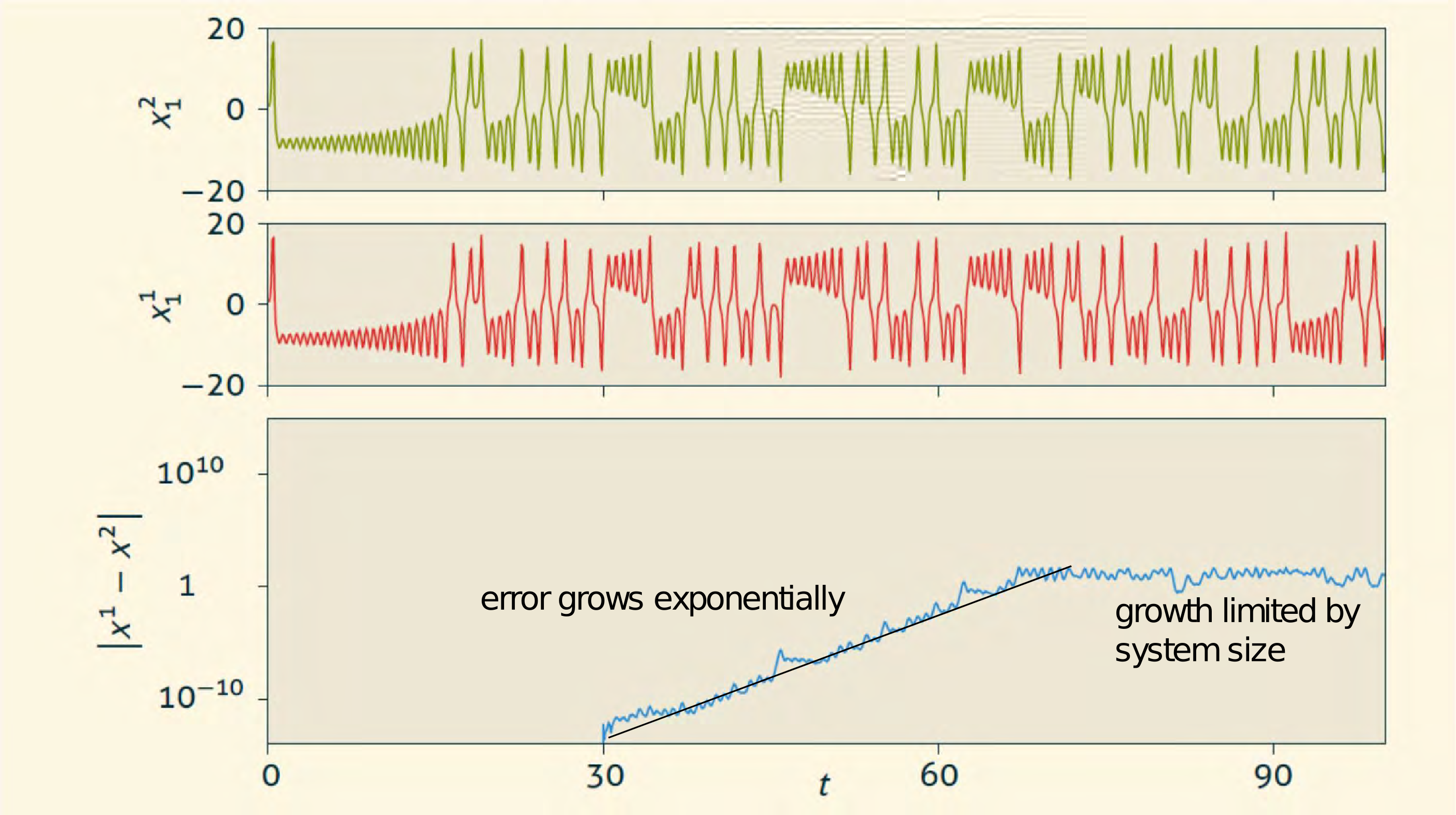
Chaotic Motion in Lorenz Attractor
Two identical Lorenz oscillators with initial conditions. Second oscillator is slightly perturbed ($10^{-14}$) at $t = 30$:
from config import (np, plt, hamiltonian,
                    plot_hamiltonian, solve_leapfrog, dt)
%matplotlib inline
N = 11

thetas = np.linspace(0, 0.99 * np.pi, 11)
ps = np.zeros_like(thetas)
plt.scatter(thetas, ps, c='b', marker='.')

plot_hamiltonian()

Time evolution
Numerical integration of equations of motion for distribution of pendulums, using leapfrog (drift+kick+drift):
n_steps = 1000
results_thetas = np.zeros((n_steps, N), dtype=np.float32)
results_thetas[0] = thetas

results_ps = np.zeros((n_steps, N), dtype=np.float32)
results_ps[0] = ps

for k in range(1, n_steps):
    results_thetas[k], results_ps[k] = solve_leapfrog(results_thetas[k - 1], results_ps[k - 1])
plt.scatter(results_thetas, results_ps, c='b', marker='.', s=1)

plot_hamiltonian()

Chaos near Unstable Fixed Point
N = 2

thetas = np.pi * np.ones(N, dtype=np.float32)
ps = np.linspace(0.01, 0.05, N)
results_thetas2 = np.zeros((n_steps, N), dtype=np.float32)
results_thetas2[0] = thetas

results_ps2 = np.zeros((n_steps, N), dtype=np.float32)
results_ps2[0] = ps

for k in range(1, n_steps):
    results_thetas2[k], results_ps2[k] = solve_leapfrog(results_thetas2[k - 1], results_ps2[k - 1])
plt.scatter(results_thetas2 % (2*np.pi), results_ps2, c='b', marker='.', s=1)
plt.scatter([np.pi], [0], c='r', marker='o')

plt.xlim(np.pi - 0.1, np.pi + 0.1)
plt.ylim(-0.01, 0.1)
plt.xlabel(r'$\theta$')
plt.ylabel(r'$p$')
Text(0, 0.5, '$p$')

$\implies$ observation near red unstable fixed point:
- phase-space trajectory becomes non-regular, obvious during subsequent passages when wrapping $\theta$ to interval $\bigl[0, 2\pi\bigr)$
Qualitative Investigation of Local Lyapunov Exponent
First around stable fixed point $\theta=0$, $p=0$ -- then around unstable fixed point $\theta=\pi$, $p=0$:
dist = 1e-10

thetas = np.pi * np.ones(N, dtype=np.float64) # change this line
ps = np.array([0.001, 0.001 + dist], dtype=np.float64)
n_steps = 100000
results_thetas3 = np.zeros((n_steps, N), dtype=np.float64)
results_thetas3[0] = thetas

results_ps3 = np.zeros((n_steps, N), dtype=np.float64)
results_ps3[0] = ps

for k in range(1, n_steps):
    results_thetas3[k], results_ps3[k] = solve_leapfrog(results_thetas3[k - 1], results_ps3[k - 1])
plt.plot(results_thetas3[:, 0], label='$p_{ini}$')
plt.plot(results_thetas3[:, 1], label='$p_{ini} + \Delta p_{ini}$')

plt.xlabel('Steps $k$')
plt.ylabel(r'$\theta$')
plt.legend();

Distance $|(\theta_2,p_2)-(\theta_1,p_1)|$
results_dist = np.sqrt(
    (results_thetas3[:, 1] - results_thetas3[:, 0])**2 +
    (results_ps3[:, 1] - results_ps3[:, 0])**2
)
plt.plot(results_dist)

plt.yscale('log')
plt.xlabel('Steps $k$')
plt.ylabel('Phase-space distance');

Frequency Diffusion
Use NAFF algorithm as early indicator of chaotic motion in periodic systems:
vs.
Further reading: "Introduction to Frequency Map Analysis" by J. Laskar in Hamiltonian Systems with Three or More Degrees of Freedom, Springer (1999), pp. 134-150
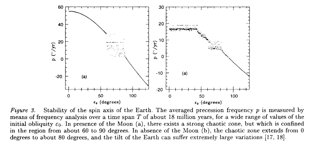
Example: Earth-Moon System
Precession of Earth is stabilised by presence of Moon:
Example: CERN LHC
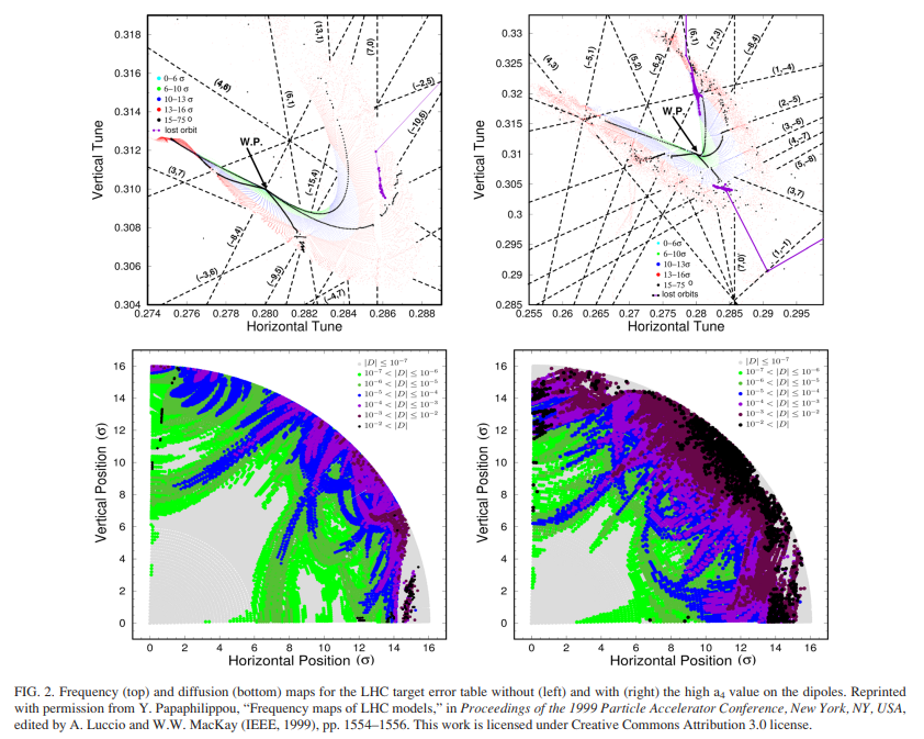
Frequency Map Analysis (FMA) to identify diffusion due to non-linear resonances:
$\implies$ always seek to maximise dynamic aperture in accelerators
$\implies$ use of "early chaos indicators" such as Lyapunov exponents or FMA: identification and mitigation/correction of sources
Try Concept on Discrete Pendulum
Can we detect frequency diffusion in discrete pendulum?
n_steps = 100000
theta_ini = np.pi - 0.001
p_ini = 0
results_thetas4 = np.zeros(n_steps, dtype=np.float64)
results_thetas4[0] = theta_ini

results_ps4 = np.zeros(n_steps, dtype=np.float64)
results_ps4[0] = p_ini

for k in range(1, n_steps):
    results_thetas4[k], results_ps4[k] = solve_leapfrog(results_thetas4[k - 1], results_ps4[k - 1])
plt.plot(results_thetas4)

plt.xlabel('Steps $k$')
plt.ylabel(r'$\theta$');

import PyNAFF
window_length = 1000

freqs_naff = []

for signal in results_thetas4.reshape((n_steps // window_length, window_length)):
    freq_naff = PyNAFF.naff(signal - np.mean(signal), turns=window_length, nterms=1)[0, 1]
    freqs_naff += [freq_naff]
plt.plot(np.arange(0, n_steps, window_length), freqs_naff, ls='none', marker='.')

plt.xlabel('Steps $k$')
plt.ylabel('NAFF determined frequency');

# plt.ylim(1.59e-2, 1.6e-2)

plt.figure(figsize=(10, 5))
plt.hist(freqs_naff);

Summing up Concepts
- sources for non-linearities in accelerators
- deterministic chaos: (bounded) deterministic dynamics with a positive Lyapunov exponent
- sensitivity to initial conditions
- prevents prediction for long-term time scales
- early indicators of chaos:
- (maximum) Lyapunov exponent
- Frequency Map Analysis (FMA)
Floating Point Representation
Represent real numbers $r\in\mathbb{R}$ on computers by "floats":
- finite and discrete set of numbers
- floating-point form: $r=\underbrace{6.022}\limits_\text{significand}\times 10{\underbrace{{}^{23}}\limits_\text{exponent}}$
Todays standard: IEEE 754
$r=\pm a \times 2^{e}$
e.g. a "single-precision" float (FP32):
- 1 sign bit
- $t=23$ bits for significand $a$
- 8 bits for exponents in range $e\in[-126, 127]$
- $\pm\infty$ and NaN
Numerical Artefacts
Floating point representation of numbers on computers $\leadsto$ numerical artefacts:
- rounding: storing the least significant bit depending on arithmetic operation
- truncating: e.g. π cannot be stored exactly but is truncated
Smallest "machine" precision in resolving real numbers: $2^{-t}$
- FP32: $2^{-23}\approx 10^{-7}$
- FP64: $2^{-52}\approx 10^{-15}$
(Drastic) Example of Truncation Error
The python library mpmath works with arbitrary numerical precision (workdps for decimal precision):
import mpmath as mp

with mp.workdps(7):
    x = mp.mpf(10) / 9   # == 1.11...

    for _ in range(30):
        print (x)
        x = (x - 1) * 10
1.111111
1.111111
1.11111
1.111104
1.111045
1.110449
1.104488
1.044884
0.4488373
-5.511627
-65.11627
-661.1627
-6621.627
-66226.27
-662272.7
-6622737.0
-6.622738e+7
-6.622738e+8
-6.622738e+9
-6.622738e+10
-6.622738e+11
-6.622738e+12
-6.622738e+13
-6.622738e+14
-6.622738e+15
-6.622738e+16
-6.622738e+17
-6.622738e+18
-6.622738e+19
-6.622738e+20
Overview: Sources of Simulation Errors
- Discretisation error
- Modelling error
- Numerical artefacts
- Input error...
Summary
- sources for non-linearities in accelerators
- deterministic chaos
- early indicators:
- (maximum) Lyapunov exponent
- Frequency Map Analysis
- numerical artefacts: rounding and truncation, machine precision
Literature
- chapter 2.1 in Justin Solomon, Numerical Algorithms