Simulation of Intense Beams in Synchrotrons

... a story of resonances and instabilities.

a notebook talk by Adrian Oeftiger $\nearrow$

in the GSI Accelerator Seminar on 3 September 2020 $\nearrow$. See also rendered talk on github $\nearrow$ and source in github repo $\nearrow$.

(hit space to go to the next slide)

Goals of this talk

• showcase new simulation suite for SIS18 and SIS100

• no theory, rather hands-on experience

• practical modelling examples with live simulations

• give overview of applications

Abstract

This introduction on collective beam dynamics focuses on high-intensity effects in synchrotrons like SIS18 or SIS100. The charged particles in the beam interact (a.) with the beam self-fields they produce and (b.) with the induced currents in the vacuum pipe. This interaction leads to corresponding collective effects, such as "space charge" (self-field interaction) or "beam coupling impedance" (interaction with the surroundings). The beam can become resonantly excited or is even driven into exponential instabilities over many revolutions in the circular accelerator. These effects potentially limit the performance, they scale with the number of particles in the beam: their understanding (and mitigation) is crucial to safely operate synchrotrons like SIS100 at highest beam intensities.

We dive into the world of these collective effects in beam physics, exploring their mechanisms and how they can lead to beam loss. During the talk, we also look behind the scenes on how to numerically model such long-term effects, in particular employing high-performance techniques such as GPU computing.

How to run this notebook at GSI:

Connect to the GSI high-performance computing cluster virgo.hpc (with port forwarding), load the accelerator physics environment and run the jupyter notebook server:

$ ssh virgo.hpc -L 8888:localhost:8888
$ singularity exec --bind /cvmfs \
    /cvmfs/vae.gsi.de/centos7/containers/user_container-develop.sif \
    bash -l
Singularity> cd /cvmfs/aph.gsi.de/
Singularity> source modules.sh
Singularity> module load aph_all
Singularity> cd
Singularity> git clone https://github.com/aoeftiger/GSI-acc-seminar-09-2020
Singularity> cd GSI-acc-seminar-09-2020
Singularity> jupyter notebook --no-browser --port=8888

... and you're ready to open your local browser and type in localhost:8888, where you open this notebook.

How to run this notebook on your individual workstation:

Install PyHEADTAIL $\nearrow$, cpymad $\nearrow$, PySixTrack $\nearrow$ and SixTrackLib $\nearrow$ in your python3 environment and run this jupyter notebook.

Note: if you don't have openCL drivers installed, replace all device=... instructions in SixTrackLib within this notebook by device=None to run on a normal single CPU thread.

Simulation of Intense Beams in Synchrotrons

... a story of resonances and instabilities.

Structure

1. PyHEADTAIL: collective beam dynamics
2. Wakefields & 1st Order Coherent Instabilities
3. SixTrackLib: symplectic non-linear 6D tracking
4. Space Charge & Resonances and 2nd Order Coherent Instabilities

Beam dynamics

3D particle motion $\leadsto$ 6 phase space coordinates: $$\mathbb{X}=(\underbrace{x, x'\vphantom{y'}}_{horizontal}, \underbrace{y, y'}_{vertical}, \underbrace{z, \delta\vphantom{y'}}_{longitudinal})$$

A beam $=$ state of $N$ macro-particles $=$ $6N$ values of phase space coordinates

Simulations:

• typically up to $\mathcal{O}(10^6)$ macro-particles
• accelerator elements to track through: up to $\mathcal{O}(1000)$
• simulations can last up to $\mathcal{O}(10^6)$ turns
• particle-to-particle interaction: binning, FFT, convolution, particle-in-cell, Poisson solvers

Requirements for simulation tools

• accurate: long-term evolution $\leadsto$ double precision
• fast: heavy number crunching $\leadsto$ high-performance computing (HPC)
  (multi-core CPU, multi-nodes (MPI) or GPU parallelisation, in particular for collective effects)
• flexible: iterative development of accelerator models with frequent updates $\leadsto$ python

The macro-particle simulation model

single-particle physics $\implies$ "tracking": particle motion due to external focusing (magnets and RF cavities)

multi-particle physics $\implies$ "collective effect kicks": direct and indirect particle-to-particle interaction

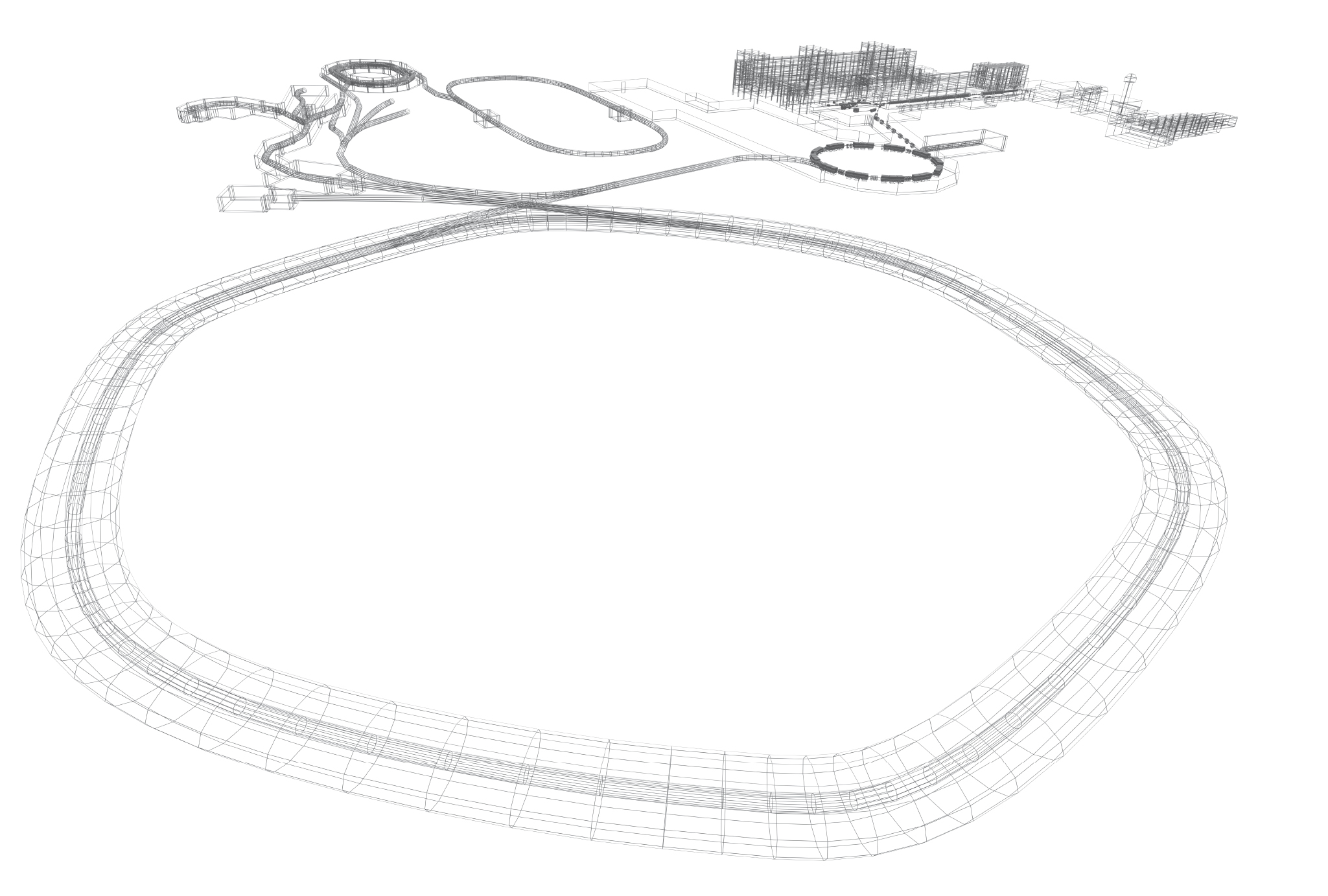
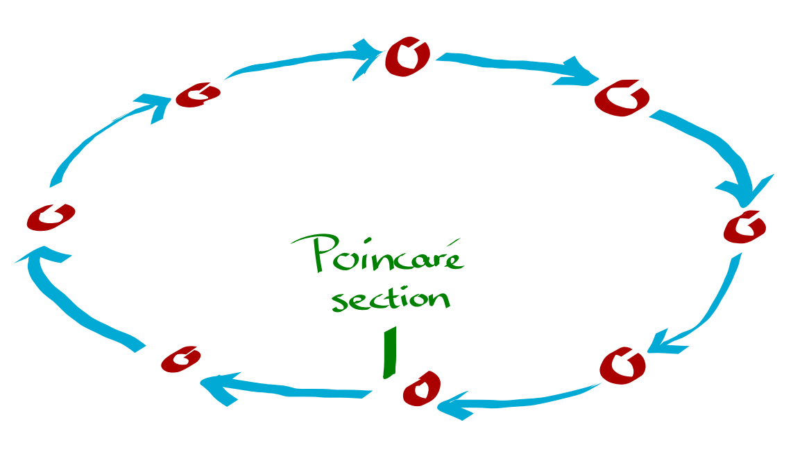Tracking around the accelerator ring

Many macro-particle codes...

... with (transverse) collective effects for synchrotrons, e.g.:

• PATRIC (GSI)
• MICROMAP (GSI)
• IMPACT (Berkeley)
• Synergia (Fermilab)
• (Py)ORBIT (SNS)
• SIMPSONS (J-PARC)
• elegant (Argonne)
• MAD-X SC (CERN)
• HEADTAIL/PyHEADTAIL (CERN, GSI)
• ...

1. PyHEADTAIL: collective beam dynamics

The PyHEADTAIL library

GPU-enabled, python based code for simulating collective beam dynamics in synchrotrons: github repo $\nearrow$

$\implies$ matrix-based transverse and non-linear longitudinal tracking

$\implies$ detailed models for collective effect kicks

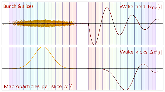
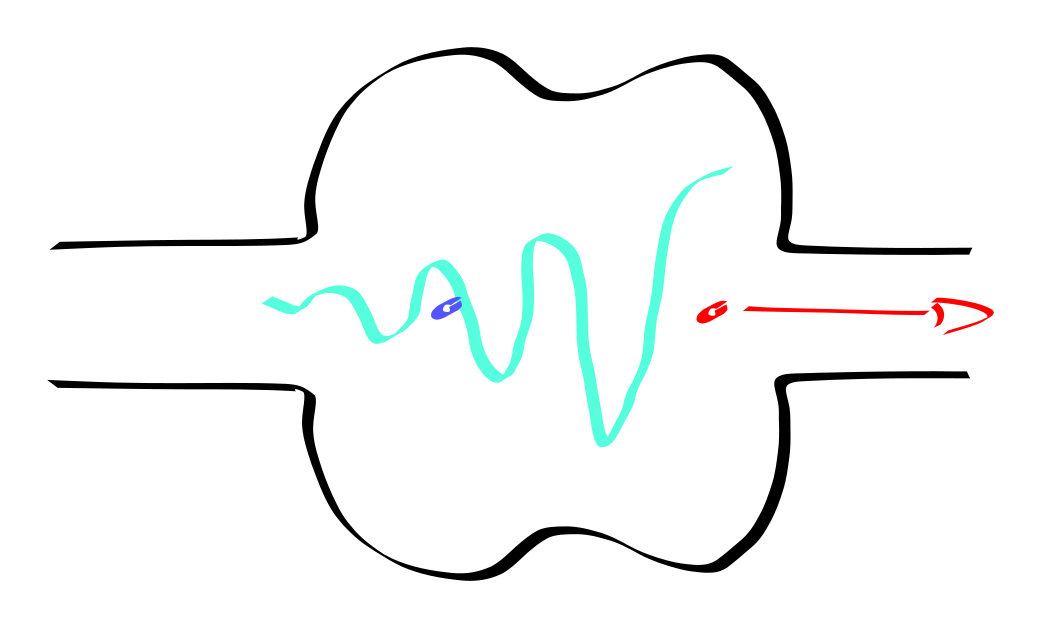Kick example: wakefield from leading particles affects trailing particles

PyHEADTAIL on one slide

• origin: C code HEADTAIL by G. Rumolo (2000), 5 PR-STAB and 2 PRL papers
• modernised PyHEADTAIL used for:
  • impedance-driven instabilities: head-tail modes, transverse mode coupling instability (TMCI), coupled-bunch instabilities, ...
  • space charge
  • electron cloud instabilities
  • mitigation techniques: feedbacks, octupoles for Landau damping, multi-harmonic RF, ...

PyHEADTAIL modules

• wakefields:
  • resistive wall
  • broad-band resonator
  • custom wake tables
• space charge
  • selfconsistent PIC
    • longitudinal, (slice-by-slice) transverse, 3D
    • open boundary Green's function (FFT)
    • open/rectangular boundary finite difference
  • frozen / adaptive field maps

• feedback (ideal and realistic [separate version])
• RF quadrupoles
• synchrotron radiation
• e-cloud pinch
• e-lens

Active development at CERN and GSI

Contributions from $>13$ developers since 2014

Resources

• PyHEADTAIL playground $\nearrow$: interactive tutorials
• Overview of PyHEADTAIL $\nearrow$: Oeftiger, A. An Overview of PyHEADTAIL. CERN-ACC-NOTE-2019-0013.
• PyHEADTAIL + SixTrackLib on GPU $\nearrow$: interactive notebook talk
• SWAN beam dynamics gallery $\nearrow$: CERN platform to launch tutorials

2. Wakefields & Dipole Moment Instabilities

PyHEADTAIL wake model

courtesy Michael Schenk

Dipole wake fields (driving impedance)

Transverse kick on slice $i$ from previous slices due to wake $W_d$:

$$\Delta x'[i] \propto \sum\limits_{j=0}^i N[j] \quad \langle x \rangle [j] \quad W_d(z[i] - z[j])$$

• no synchrotron motion:

  • kicks accumulate, linac-like beam breakup

• with synchrotron motion: feedback loop

  • chroma $Q'=0$:
    • synchrotron sidebands separate $\rightarrow$ stable beam
    • synchrotron sidebands couple $\rightarrow$ transverse mode coupling instability
  • chroma $Q'\neq 0$: head-tail instability

Simulating head-tail instability in SIS100

$\rightarrow$ use PyHEADTAIL to simulate head-tail instability due to resistive wall impedance of SIS100 vacuum tube:

# set up plotting etc
from imports import *

Importing PyHEADTAIL:

import PyHEADTAIL

PyHEADTAIL v1.14.1.28 (commit gc108ffeac6)

Setting up tracking around the SIS100 ring

Transverse tracking:

from PyHEADTAIL.trackers.transverse_tracking import TransverseMap
from PyHEADTAIL.trackers.detuners import Chromaticity

from pyheadtail_setup import transverse_map_kwargs, Q_x, Q_y
print ('chosen horizontal tune: {:.2f}, vertical tune: {:.2f}'.format(Q_x, Q_y))

chosen horizontal tune: 18.84, vertical tune: 18.73

Low, slightly positive chromaticity below transition $=$ strong growth rate of rigid bunch mode

transverse_map = TransverseMap(
    detuners=[Chromaticity(
        Qp_x=5, Qp_y=5)],
    **transverse_map_kwargs,
)

Longitudinal tracking:

from PyHEADTAIL.trackers.longitudinal_tracking import RFSystems

from pyheadtail_setup import longitudinal_map_kwargs

longitudinal_map = RFSystems(**longitudinal_map_kwargs)

Setting up collective effect kick

Simulate wakefields in bunch via circular resistive wall model:

from PyHEADTAIL.impedances.wakes import WakeField, CircularResistiveWall
from PyHEADTAIL.particles.slicing import UniformBinSlicer

# responsible for binning the beam longitudinally:
slicer = UniformBinSlicer(n_slices=40, n_sigma_z=3)

resistive_wall_wake = CircularResistiveWall(
    pipe_radius=0.03,
    resistive_wall_length=longitudinal_map_kwargs['circumference'],
    conductivity=1.4e6,
    dt_min=None,
    n_turns_wake=1, 
)
wakefield = WakeField(slicer, resistive_wall_wake)

Assembling the map around the SIS100 ring:

pyht_ring_elements = list(transverse_map) + [longitudinal_map, wakefield]

Initialising the particle bunch

from PyHEADTAIL.particles.generators import generate_Gaussian6DTwiss

from pyheadtail_setup import beam_kwargs

n_macroparticles = 2000
intensity = 6.25e10

np.random.seed(0)

pyht_beam = generate_Gaussian6DTwiss(
    macroparticlenumber=n_macroparticles,
    intensity=intensity,
    **beam_kwargs,
    **transverse_map.get_injection_optics(
        for_particle_generation=True),
)

We'll give the bunch an initial kick:

pyht_beam.y += 0.1 * pyht_beam.sigma_y()

slices0 = pyht_beam.get_slices(slicer, statistics=['mean_y'])

resistive_wall_wake.dt_min = slices0.convert_to_time(slices0.slice_widths[0])

Let's go – simulating SIS100 in PyHEADTAIL:

n_turns = 10000

my = np.zeros(n_turns, dtype=float)

# loop over turns
for i in range(n_turns):
    # loop over elements around ring
    for element in pyht_ring_elements:
        element.track(pyht_beam)

    # record vertical bunch centroid amplitude
    my[i] = pyht_beam.mean_y()

Outcome of our simulation?

plt.plot(my * 1e3)
plt.xlabel('Turns')
plt.ylabel(r'$\langle y \rangle$ [mm]')
plt.title('Vertical bunch centroid motion');

$\leadsto$ centre-of-mass of the bunch grows exponentially $\implies$ instability!

Let's fit the exponential growth rate:

growth_rate, _ = np.polyfit(np.arange(n_turns), np.log(my**2) / 2., 1)

print ('growth time: {:.0f} turns ~ {:.3f} sec'.format(
    1 / growth_rate, 1083.6 / (0.567 * 3e8) / growth_rate))

growth time: 1963 turns ~ 0.013 sec

plt.plot(my * 1e3)
plt.plot(np.arange(n_turns), 
         max(abs(my[:10]))* 0.8 * 1e3 * 
         np.exp(growth_rate * np.arange(n_turns)),
         ls='--')
plt.xlabel('Turns')
plt.ylabel(r'$\langle y \rangle$ [mm]')
plt.title('Vertical bunch centroid motion');

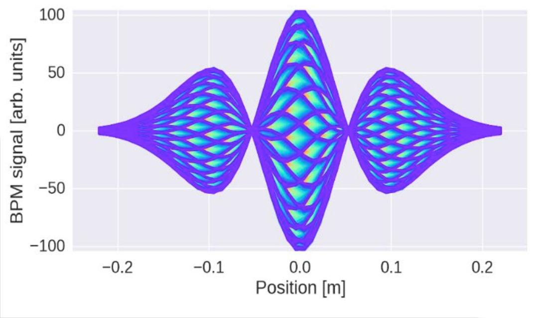
from imports import plot_intrabunch

plot_intrabunch(pyht_ring_elements, pyht_beam, slicer, slices0)

$\implies$ indeed a rigid bunch mode, no nodes!

Common mitigation strategies for head-tail instabilities

1. change chromaticity: sextupole magnets
2. Landau damping: octupole magnets
3. linear coupling: skew quadrupole magnets
4. active transverse feedback (damper)

Mitigation 1: Chromaticity

• higher-order modes $=$ lower growth rate
• for below (above) transition $\rightarrow$ go to negative (positive) chromaticity
• mode growth rates e.g. from Sacherer approach (1974)

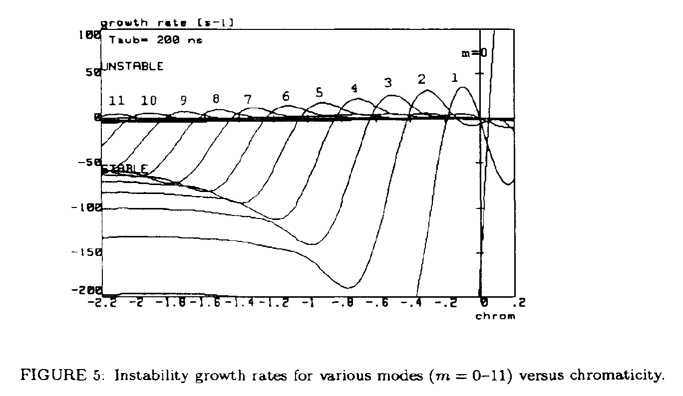example CERN PS
taken from R. Cappi, Observation of high-order head-tail instabilities at the CERN-PS, CERN/PS 95-02

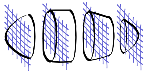
Mitigation 2: Octupoles

• detuning with transverse amplitude $=$ tune spread $\leadsto$ Landau damping
• dispersion relations to solve for stability diagrams

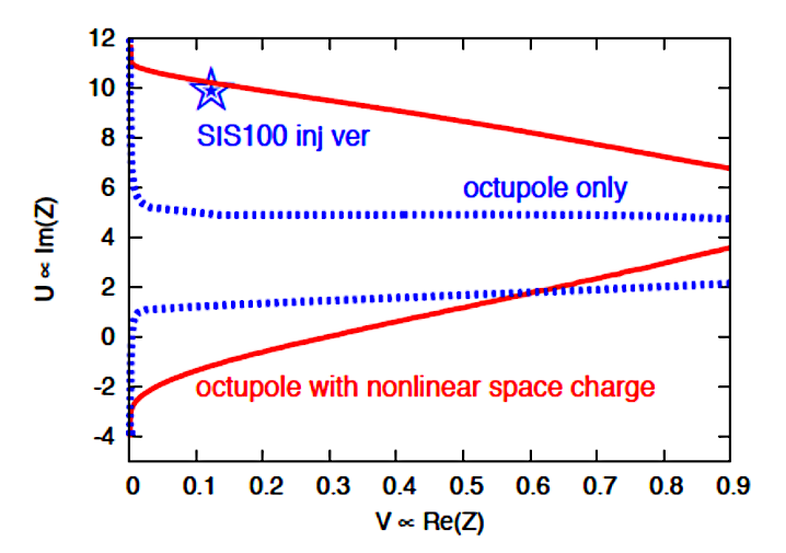V. Kornilov on MAC20b or PRSTAB 11, 014201 (2008)

Mitigation 3: Coupling

• mix growth rates of transverse planes (e.g. CERN PS)
• "share" Landau damping

See e.g. Métral, E. Theory of coupled Landau damping. Part. Accel., 62 (1999) 259. $\nearrow$

Mitigation 4: Damper

Let's use the foreseen SIS100 damper with $100$ turns $\nearrow$ to stabilise the previously simulated head-tail instability:

from PyHEADTAIL.feedback.transverse_damper import TransverseDamper

damper = TransverseDamper(dampingrate_x=100, dampingrate_y=100)

Dampers active

pyht_ring_elements += [damper]

Continue simulation with damper on now:

n_turns_2 = 1000

my_2 = np.zeros(n_turns_2, dtype=float)

# loop over turns
for i in range(n_turns_2):
    # loop over elements around ring
    for element in pyht_ring_elements:
        element.track(pyht_beam)

    # record vertical bunch centroid amplitude
    my_2[i] = pyht_beam.mean_y()

Outcome of our follow-up simulation?

plt.plot(np.concatenate((my, my_2)) * 1e3)
plt.axvline(n_turns, color='black', ls='--')
plt.text(n_turns, plt.ylim()[1] * 0.9, r'damper on $\rightarrow$ ',
         fontsize=20, ha='right', va='top', bbox={'facecolor': 'white', 'alpha': 0.5})
plt.xlabel('Turns')
plt.ylabel(r'$\langle y \rangle$ [mm]')
plt.title('Vertical bunch centroid motion');

$\implies$ stabilised beam!

$\leadsto$ important: these PyHEADTAIL simulations are kept simple to be instructive, same model can be extended and used in higher resolution for proper study!

More on PyHEADTAIL

Potentially interesting for GSI:

• realistic feedback model implemented in PyHEADTAIL on branch feature/multibunch_feedback $\nearrow$:
  • bunch-by-bunch feedback
  • includes many engineering filters
  • how-to talk by J. Komppula $\nearrow$
  • used e.g. to simulate real LHC ADT damper module
  • Komppula, J., et al. Simulation Tools for the Design and Performance Evaluation of Transverse Feedback Systems. (IPAC 2017). $\nearrow$

• handy, advanced space charge models:
  • for simulation on coherent stability with self-consistent space charge: slice-by-slice recentring models with aperture on grid boundary to remove invalid particles
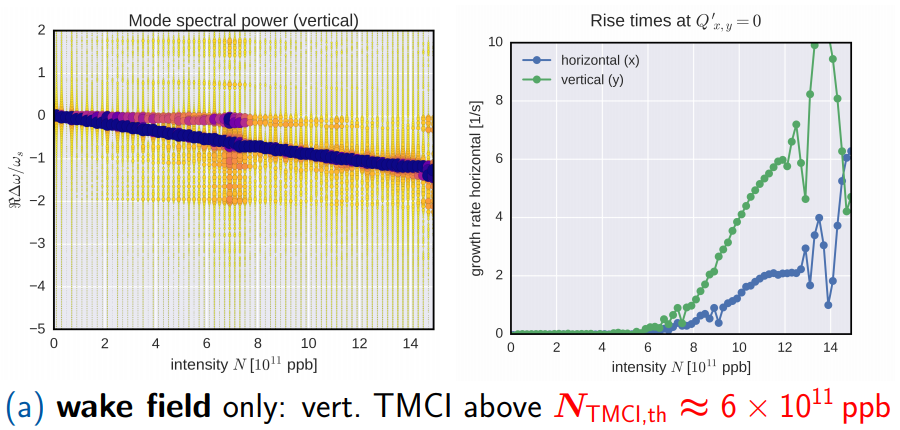
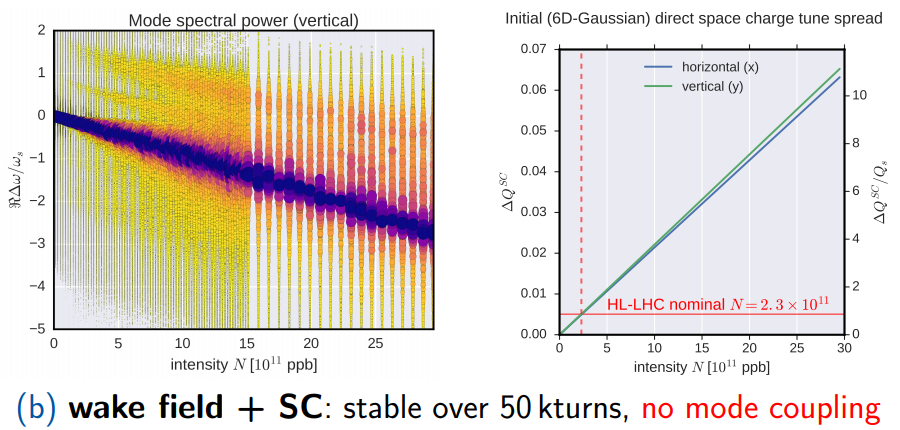
  • used e.g. to simulate space charge impact on TMCI thresholds in LHC and SPS at CERN, see e.g. Poster on LHC Instabilities $\nearrow$ and Métral, E., Oeftiger, A. et al. Space Charge and Transverse Instabilities at the CERN SPS and LHC. (IPAC 2019). $\nearrow$

3. SixTrackLib: symplectic non-linear 6D tracking

The SixTrackLib library

GPU-enabled C templated code with Python API for simulating single-particle beam dynamics: github repo $\nearrow$

$\implies$ advanced non-linear thin-lens tracking, no further approximations

$\implies$ approximative / simplified models for collective effect kicks:

• fixed frozen space charge
• 4D and 6D beam-beam

Example for tracking: dipoles and (de-)focusing quadrupoles

Background of SixTrackLib

• origin: Fortran77/90 code SixTrack $\nearrow$:
  • numerically portable across OS and architectures
  • used via volunteer computing project LHC@Home $\nearrow$ with $>200$k registered users and $>20$k simultaneously available CPU cores
• modernised SixTrackLib written from scratch by R. de Maria and M. Schwinzerl
  • standalone library
  • in future to be integrated into SixTrack as new core
  • supports GPUs via openCL and CUDA

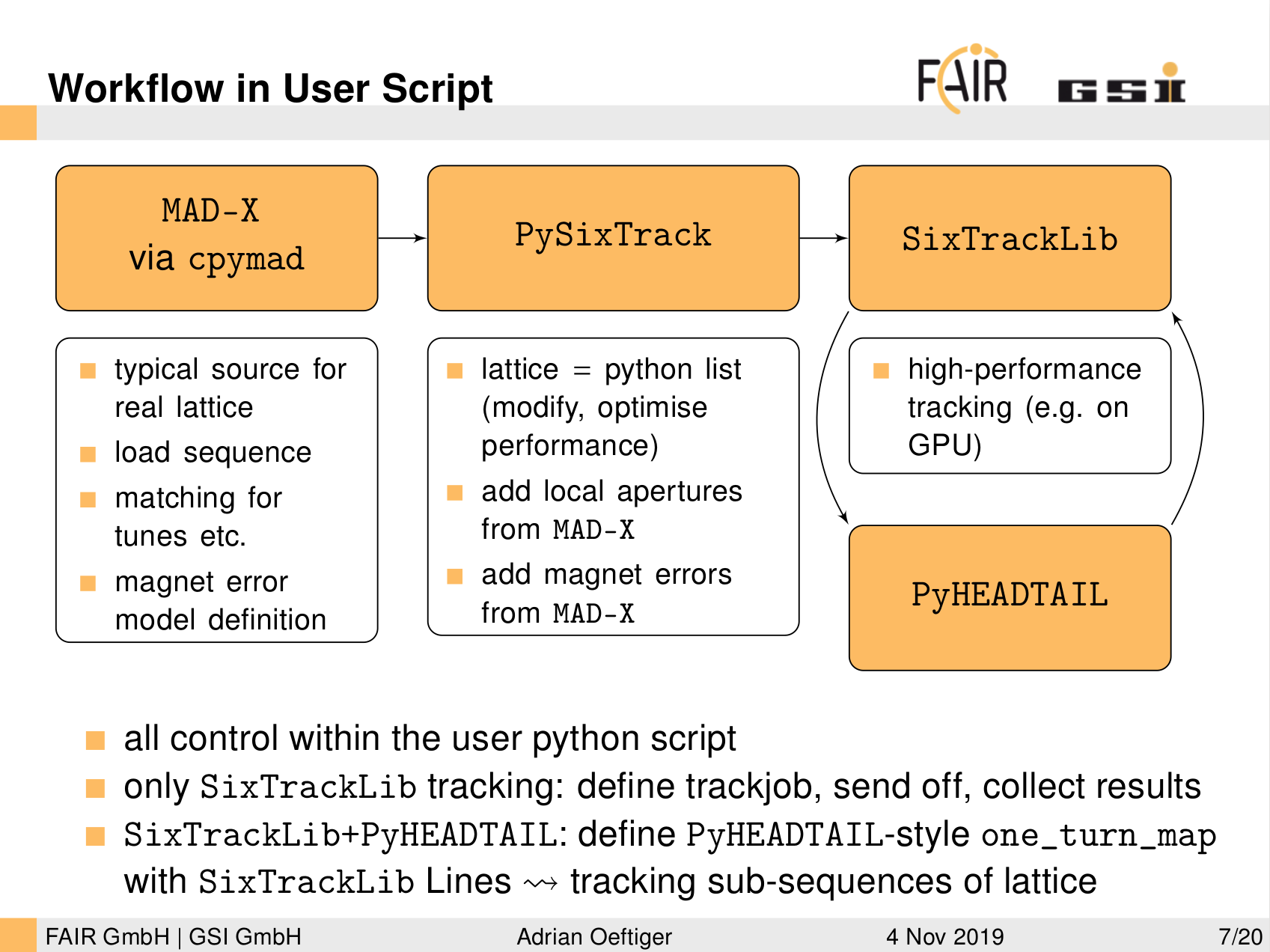
import pysixtrack
import sixtracklib as stl

from cpymad.madx import Madx

MAD-X part first

madx = Madx()
madx.options.echo = False
madx.options.warn = False
madx.options.info = False

  ++++++++++++++++++++++++++++++++++++++++++++
  +     MAD-X 5.06.00  (64 bit, Linux)       +
  + Support: mad@cern.ch, http://cern.ch/mad +
  + Release   date: 2020.08.13               +
  + Execution date: 2020.09.03 14:30:51      +
  ++++++++++++++++++++++++++++++++++++++++++++

Define SIS100 lattice in MAD-X:

madx.call('./SIS100.seq')

Define SIS100 U${}^{28+}$ beam in MAD-X:

from sixtracklib_setup import *

print ('mass = {:d}amu, charge = {:d}e, Ekin = {:.0f}MeV/u'.format(
    A, Q, 1e-6 * Ekin_per_nucleon))

mass = 238amu, charge = 28e, Ekin = 200MeV/u

madx.command.beam(particle='ion', mass=A*nmass, charge=Q, energy=Etot);

madx.input('''
            kqd := -0.2798446835;
            kqf := 0.2809756135;

            K1NL_S00QD1D :=  kqd ;
            K1NL_S00QD1F :=  kqf ;
            K1NL_S00QD2F :=  kqf ;
            K1NL_S52QD11 :=  1.0139780 * kqd ;
            K1NL_S52QD12 :=  1.0384325 * kqf ;
        ''');

madx.use(sequence='sis100ring')

assert madx.command.select(
    flag='MAKETHIN',
    class_='QUADRUPOLE',
    slice_='9',
)

assert madx.command.select(
    flag='MAKETHIN',
    class_='SBEND',
    slice_='9',
)

assert madx.command.makethin(
    makedipedge=True,
    style='teapot',
    sequence='SIS100RING',
)

makethin: style chosen : teapot
makethin: slicing sequence : sis100ring

Match tunes to $Q_x=18.84$, $Q_y=18.73$:

madx.use(sequence='sis100ring')

madx.input('''
match, sequence=SIS100RING;
global, sequence=SIS100RING, q1=18.84, q2=18.73;
vary, name=kqf, step=0.00001;
vary, name=kqd, step=0.00001;
lmdif, calls=500, tolerance=1.0e-10;
endmatch;
''');

START MATCHING

number of sequences: 1
sequence name: sis100ring
number of variables:    2
user given constraints: 2
total constraints:      2

START LMDIF:

Initial Penalty Function =   0.11937828E-03


call:       4   Penalty function =   0.20839228E-12
 ++++++++++ LMDIF ended: converged successfully
call:       4   Penalty function =   0.20839228E-12

MATCH SUMMARY

Node_Name                  Constraint   Type  Target Value       Final Value        Penalty
--------------------------------------------------------------------------------------------------
Global constraint:         q1           4     1.88400000E+01     1.88400000E+01     1.18091011E-13
Global constraint:         q2           4     1.87300000E+01     1.87300000E+01     9.03012738E-14


Final Penalty Function =   2.08392285e-13





Variable                 Final Value  Initial Value Lower Limit  Upper Limit 
--------------------------------------------------------------------------------
kqf                       2.80985e-01  2.80976e-01 -1.00000e+20  1.00000e+20
kqd                      -2.79854e-01 -2.79845e-01 -1.00000e+20  1.00000e+20

END MATCH SUMMARY

VARIABLE "TAR" SET TO   2.08392285e-13

twiss = madx.twiss();

print ('\nQ1 = {:.2f} and Q2 = {:.2f}'.format(
    twiss.summary['q1'], twiss.summary['q2']))

enter Twiss module
  
iteration:   1 error:   0.000000E+00 deltap:   0.000000E+00
orbit:   0.000000E+00  0.000000E+00  0.000000E+00  0.000000E+00  0.000000E+00  0.000000E+00

++++++ table: summ

            length             orbit5               alfa            gammatr 
            1083.6                 -0      0.00421942094        15.39478305 

                q1                dq1            betxmax              dxmax 
       18.84000003       -39.80862552        19.95869544        3.138851059 

             dxrms             xcomax             xcorms                 q2 
       1.400134289                  0                  0        18.72999997 

               dq2            betymax              dymax              dyrms 
      -39.71522141        21.30590028                  0                  0 

            ycomax             ycorms             deltap            synch_1 
                 0                  0                  0                  0 

           synch_2            synch_3            synch_4            synch_5 
                 0                  0                  0                  0 

           synch_6            synch_8             nflips 
                 0                  0                  0 

Q1 = 18.84 and Q2 = 18.73

Now transfer SIS100 lattice to PySixTrack

pysixtrack_elements = pysixtrack.Line.from_madx_sequence(
    madx.sequence.sis100ring, 
    exact_drift=True, install_apertures=False,
)

pysixtrack_elements.elements is a python list, we can play with it...

Finally go to SixTrackLib

Transfer lattice from PySixTrack:

elements = stl.Elements.from_line(pysixtrack_elements)

nturns = 2**16
elements.BeamMonitor(num_stores=nturns);

And define particle set:

npart = 1
particles = stl.Particles.from_ref(npart, p0c=p0c)

particles.x += 1e-6
particles.y += 1e-6

The trackjob will define the simulation kernel for us:

job = stl.TrackJob(elements, particles, device=None)

$\leadsto$ note the device argument:

this can be 'opencl:0.0' for openCL parallelisation, e.g. for multi-core CPU or GPU!

Let's track to confirm the tunes from MAD-X:

job.track_until(nturns)
job.collect()

Evaluation:

rec_x = job.output.particles[0].x
rec_y = job.output.particles[0].y

plt.plot(rec_x[:128])
plt.plot(rec_y[:128])

[<matplotlib.lines.Line2D at 0x7f6e2c626f90>]

from sixtracklib_setup import plot_tunes_from_stl_results

plot_tunes_from_stl_results(twiss, job)

$\implies$ tunes are on top of MAD-X, perfect!

4. Space Charge & Resonances and 2nd Order Coherent Instabilities

SixTrackLib provides extremely fast simulations!

Including in the SIS100 model

• full lattice (from gitlab repo $\nearrow$)
• non-linear, frozen 3D space charge
• field error models until 7th order for dipole and quadrupole magnets

$~\longrightarrow~$ scan 2D tune diagrams, $\approx 2$min per simulation for 20'000 turns

(on virgo.hpc cluster: 64 CPU cores or NVIDIA V100 GPU)

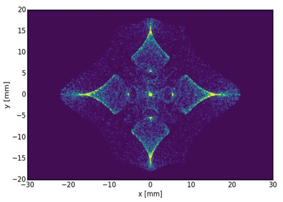
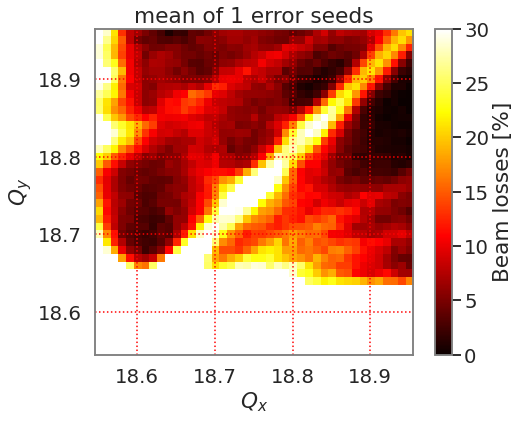
Non-linear magnet resonances + space charge

$~\Longrightarrow~$ study space charge limit in SIS100 for heavy-ion cycles:

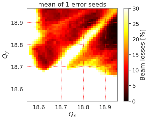beam loss tune diagram for SIS100

Mitigation techniques

1. correcting beta-beat
2. double harmonic RF for bunch flattening
3. electron lenses (to be studied)

Mitigation 1: Correcting Beta-beat

No gradient errors in the quadrupole magnets (but all other non-linear field errors):

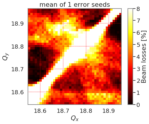beam loss tune diagram for SIS100

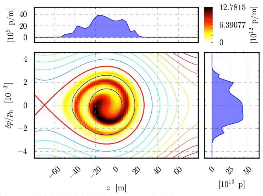
Mitigation 2: Double Harmonic RF

Double harmonic $\implies$ flattened bunch profile $\implies$ weaker space charge $\implies$ more space in tune diagram

Comparison of bunch profiles:

$\implies$ 0.8 smaller space charge tune spread!

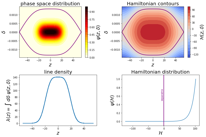
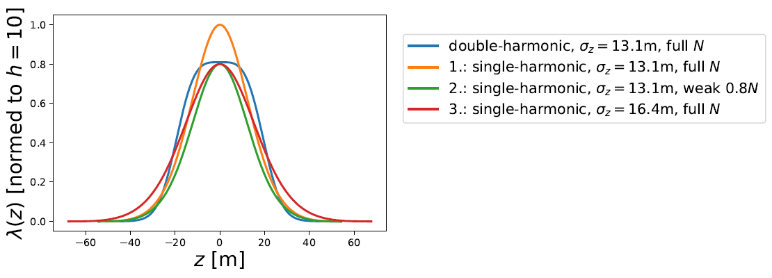
Results:

single harmonic

double harmonic

Compare space charge resonance behaviour

With the new merger SixHead $=$ SixTrackLib + PyHEADTAIL on the GPU:

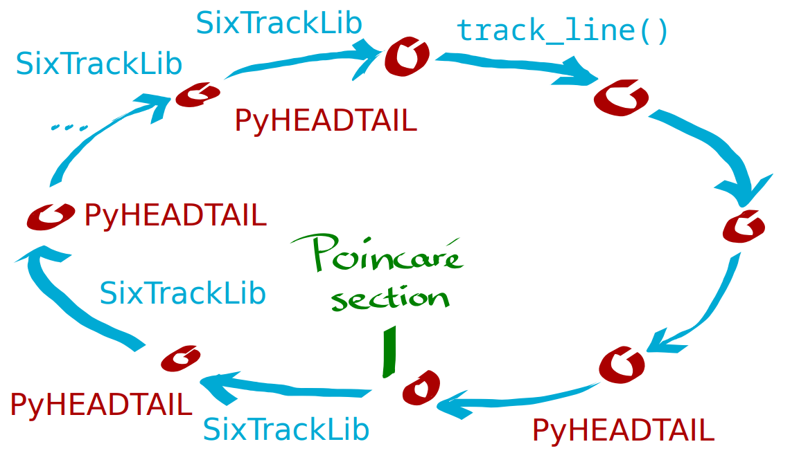Alternating SixTrackLib tracking and PyHEADTAIL kicking

Approach:

for i in range(n_turns):
    # SixTrackLib:
    pyht_to_stl()
    trackjob.track_until(i)
    stl_to_pyht()
    # PyHEADTAIL
    spacecharge.track(pyht_beam)

$\implies$ compare frozen space charge models with self-consistent 3D particle-in-cell space charge:

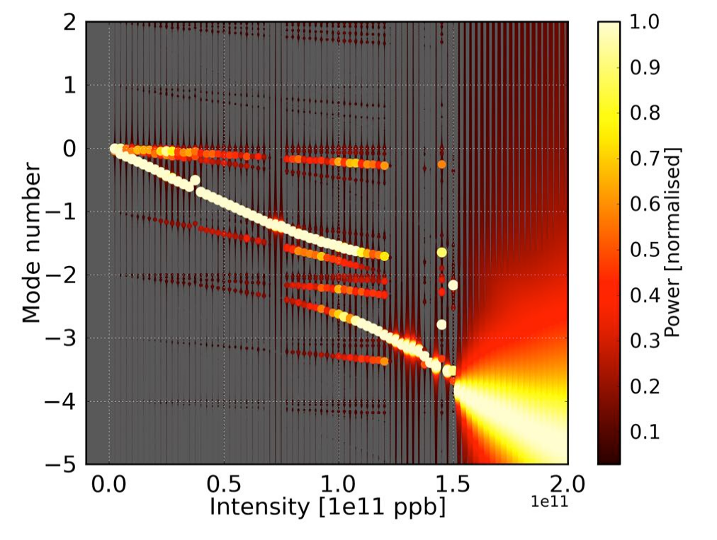
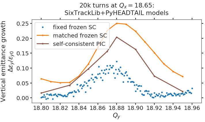1D tune scan across resonance

2nd (and higher) order coherent instabilities

courtesy Ingo Hofmann

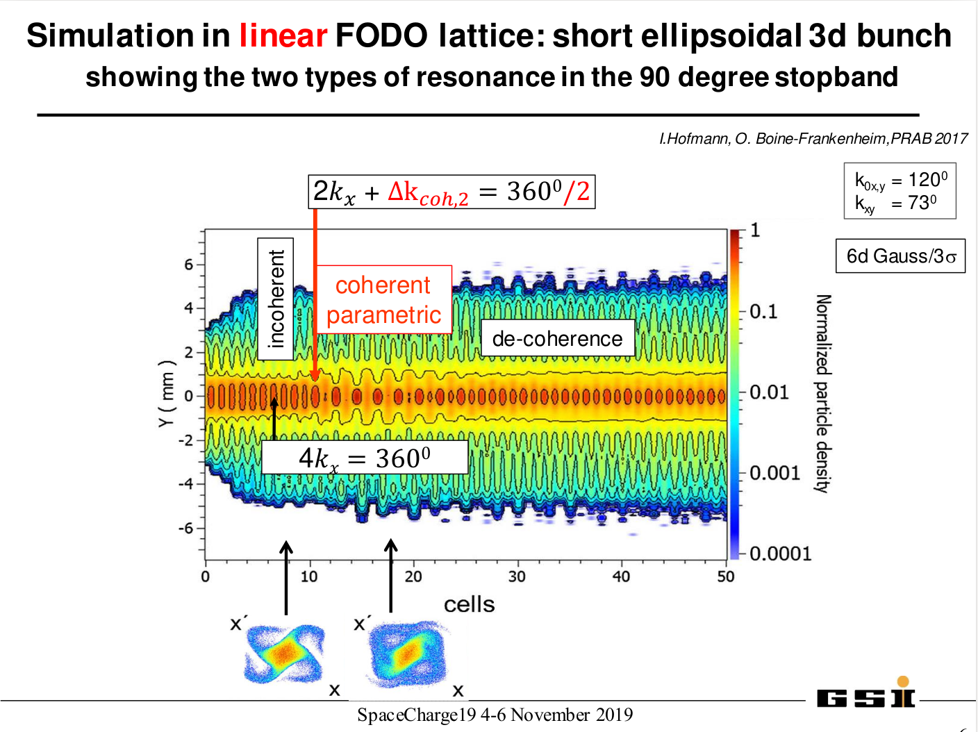
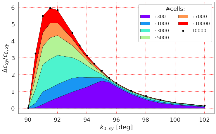
The $90^\circ$ stop-band

Investigating 90deg stop-band with SixHead:

• full 3D selfconsistent study, including synchrotron motion
• characterise higher-order coherent instabilities in synchrotrons
• 10'000 turns on GPU with 4 million macro-particles in $<4$h

1D tune scan across resonance for 300x slower $Q_s$ than $Q_{x,y}$

... so long and thanks for all the fish ...

Summary

New suite SixHead consisting of:

• symplectic 6D non-linear tracking with SixTrackLib
• collective beam dynamics with PyHEADTAIL (wakefields, space charge, feedbacks, ...)

is parallelised on:

• multi-core CPU (tracking)
• GPU

and renders possible:

• accurate, fast and flexible simulation studies for SIS18 and SIS100 for high-intensity operation

Thank you for your attention!

Acknowledgements

CERN collaborators: R. de Maria, H. Bartosik, M. Schwinzerl

GSI colleagues: V. Chetvertkova, S. Sorge